Downloaded 10 times
![2.14 Analysis and Design of Feedback Control Systems
State-Space Representation of LTI Systems
Derek Rowell
October 2002
1 Introduction
The classical control theory and methods (such as root locus) that we have been using in
class to date are based on a simple input-output description of the plant, usually expressed
as a transfer function. These methods do not use any knowledge of the interior structure of
the plant, and limit us to single-input single-output (SISO) systems, and as we have seen
allows only limited control of the closed-loop behavior when feedback control is used.
Modern control theory solves many of the limitations by using a much “richer” description
of the plant dynamics. The so-called state-space description provide the dynamics as a set
of coupled first-order differential equations in a set of internal variables known as state
variables, together with a set of algebraic equations that combine the state variables into
physical output variables.
1.1 Definition of System State
The concept of the state of a dynamic system refers to a minimum set of variables, known
as state variables, that fully describe the system and its response to any given set of inputs
[1-3]. In particular a state-determined system model has the characteristic that:
A mathematical description of the system in terms of a minimum set of variables
xi(t), i = 1, . . . , n, together with knowledge of those variables at an initial time t0
and the system inputs for time t ≥ t0, are sufficient to predict the future system
state and outputs for all time t > t0.
This definition asserts that the dynamic behavior of a state-determined system is completely
characterized by the response of the set of n variables xi(t), where the number n is defined
to be the order of the system.
The system shown in Fig. 1 has two inputs u1(t) and u2(t), and four output vari-
ables y1(t), . . . , y4(t). If the system is state-determined, knowledge of its state variables
(x1(t0), x2(t0), . . . , xn(t0)) at some initial time t0, and the inputs u1(t) and u2(t) for t ≥ t0 is
sufficient to determine all future behavior of the system. The state variables are an internal
description of the system which completely characterize the system state at any time t, and
from which any output variables yi(t) may be computed.
Large classes of engineering, biological, social and economic systems may be represented
by state-determined system models. System models constructed with the pure and ideal
(linear) one-port elements (such as mass, spring and damper elements) are state-determined
1](https://image.slidesharecdn.com/statespace-190115163537/75/State-space-courses-1-2048.jpg)

![where ˙xi = dxi/dt and each of the functions fi (x, u, t), (i = 1, . . . , n) may be a general
nonlinear, time varying function of the state variables, the system inputs, and time. 1
It is common to express the state equations in a vector form, in which the set of n state
variables is written as a state vector x(t) = [x1(t), x2(t), . . . , xn(t)]T
, and the set of r inputs
is written as an input vector u(t) = [u1(t), u2(t), . . . , ur(t)]T
. Each state variable is a time
varying component of the column vector x(t).
This form of the state equations explicitly represents the basic elements contained in
the definition of a state determined system. Given a set of initial conditions (the values of
the xi at some time t0) and the inputs for t ≥ t0, the state equations explicitly specify the
derivatives of all state variables. The value of each state variable at some time ∆t later may
then be found by direct integration.
The system state at any instant may be interpreted as a point in an n-dimensional state
space, and the dynamic state response x(t) can be interpreted as a path or trajectory traced
out in the state space.
In vector notation the set of n equations in Eqs. (1) may be written:
˙x = f (x, u, t) . (2)
where f (x, u, t) is a vector function with n components fi (x, u, t).
In this note we restrict attention primarily to a description of systems that are linear and
time-invariant (LTI), that is systems described by linear differential equations with constant
coefficients. For an LTI system of order n, and with r inputs, Eqs. (1) become a set of n
coupled first-order linear differential equations with constant coefficients:
˙x1 = a11x1 + a12x2 + . . . + a1nxn + b11u1 + . . . + b1rur
˙x2 = a21x1 + a22x2 + . . . + a2nxn + b21u1 + . . . + b2rur
...
...
˙xn = an1x1 + an2x2 + . . . + annxn + bn1u1 + . . . + bnrur
(3)
where the coefficients aij and bij are constants that describe the system. This set of n
equations defines the derivatives of the state variables to be a weighted sum of the state
variables and the system inputs.
Equations (8) may be written compactly in a matrix form:
d
dt
x1
x2
...
xn
=
a11 a12 . . . a1n
a21 a22 . . . a2n
...
...
an1 an2 . . . ann
x1
x2
...
xn
+
b11 . . . b1r
b21 b2r
...
...
bn1 . . . bnr
u1
...
ur
(4)
which may be summarized as:
˙x = Ax + Bu (5)
1
In this note we use bold-faced type to denote vector quantities. Upper case letters are used to denote
general matrices while lower case letters denote column vectors. See Appendix A for an introduction to
matrix notation and operations.
3](https://image.slidesharecdn.com/statespace-190115163537/75/State-space-courses-3-2048.jpg)


![and substitute into the Laplace transform of the output equation Y (s) = cX(s)+
dU(s):
Y (s) =
bc
s − a
+ d U(s)
=
ds + (bc − ad)
(s − a)
U(s) (vi)
The transfer function is:
H(s) =
Y (s)
U(s)
=
ds + (bc − ad)
(s − a)
. (vii)
The differential equation is found directly:
(s − a) Y (s) = (ds + (bc − ad)) U(s), (viii)
and rewriting as a differential equation:
dy
dt
− ay = d
du
dt
+ (bc − ad) u(t). (ix)
Classical representations of higher-order systems may be derived in an analogous set of
steps by using the Laplace transform and matrix algebra. A set of linear state and output
equations written in standard form
˙x = Ax + Bu (13)
y = Cx + Du (14)
may be rewritten in the Laplace domain. The system equations are then
sX(s) = AX(s) + BU(s)
Y(s) = CX(s) + DU(s) (15)
and the state equations may be rewritten:
sx(s) − Ax(s) = [sI − A] x(s) = Bu(s). (16)
where the term sI creates an n×n matrix with s on the leading diagonal and zeros elsewhere.
(This step is necessary because matrix addition and subtraction is only defined for matrices
of the same dimension.) The matrix [sI − A] appears frequently throughout linear system
theory; it is a square n × n matrix with elements directly related to the A matrix:
[sI − A] =
(s − a11) −a12 · · · −a1n
−a21 (s − a22) · · · −a2n
...
...
...
...
−an1 −an2 · · · (s − ann)
. (17)
8](https://image.slidesharecdn.com/statespace-190115163537/75/State-space-courses-8-2048.jpg)

![capacitor voltage vC(t) and the inductor current iL(t) as state variables, and
generates the following pair of state equations:
˙vc
˙iL
=
0 1/C
−1/L −R/L
vc
iL
+
0
1/L
Vin. (i)
The required output equation is:
y(t) = 1 0
vc
iL
+ 0 Vin (ii)
Step 1: In Laplace transform form the state equations are:
sVC(s) = 0VC(s) + 1/CIL(s) + 0Vs(s)
sIL(s) = −1/LVC(s) − R/LIL(s) + 1/LVs(s) (iii)
Step 2: Reorganize the state equations:
sVC(s) − 1/CIL(s) = 0Vs(s) (iv)
1/LVC(s) + [s + R/L] IL(s) = 1/LVs(s) (v)
Step 3: In this case we have two simultaneous operational equations in the state
variables vC and iL. The output equation requires only vC. If Eq. (iv) is
multiplied by [s + R/L], and Eq. (v) is multiplied by 1/C, and the equations
added, IL(s) is eliminated:
[s (s + R/L) + 1/LC] VC(s) = 1/LCVs(s) (vi)
Step 4: The output equation is y = vC. Operate on both sides of Eq. (vi) by
[s2
+ (R/L)s + 1/LC]
−1
and write in quotient form:
VC(s) =
1/LC
s2 + (R/L)s + 1/LC
Vs(s) (vii)
Step 5: The transfer function H(s) = Vc(s)/Vs(s) is:
H(s) =
1/LC
s2 + (R/L)s + 1/LC
(viii)
Step 6: The differential equation relating vC to Vs is:
d2
vC
dt2
+
R
L
dvC
dt
+
1
LC
vC =
1
LC
Vs(t) (ix)
10](https://image.slidesharecdn.com/statespace-190115163537/75/State-space-courses-10-2048.jpg)
![Cramer’s Rule, for the solution of a set of linear algebraic equations, is a useful method
to apply to the solution of these equations. In solving for the variable xi in a set of n linear
algebraic equations, such as Ax = b the rule states:
xi =
det A(i)
det [A]
(18)
where A(i)
is another n × n matrix formed by replacing the ith column of A with the vector
b.
If
[sI − A] X(s) = BU(s) (19)
then the relationship between the ith state variable and the input is
Xi(s) =
det [sI − A](i)
det [sI − A]
U(s) (20)
where (sI − A)(i)
is defined to be the matrix formed by replacing the ith column of (sI − A)
with the column vector B. The differential equation is
det [sI − A] xi = det (sI − A)(i)
uk(t). (21)
Example 4
Use Cramer’s Rule to solve for vL(t) in the electrical system of Example 3.
Solution: From Example 3 the state equations are:
˙vc
˙iL
=
0 1/C
−1/L −R/L
vc
iL
+
0
1/L
Vin(t) (i)
and the output equation is:
vL = −vC − RiL + Vs(t). (ii)
In the Laplace domain the state equations are:
s −1/C
1/L s + R/L
Vc(s)
IL(s)
=
0
1/L
Vin(s). (iii)
11](https://image.slidesharecdn.com/statespace-190115163537/75/State-space-courses-11-2048.jpg)
![The voltage VC(s) is given by:
VC(s) =
det (sI − A)(1)
det [(sI − A)]
Vin(s) =
det
0 −1/C
1/L (s + R/L)
det
s −1/C
1/L (s + R/L)
Vin(s)
=
1/LC
s2 + (R/L)s + (1/LC)
Vin(s). (iv)
The current IL(t) is:
IL(s) =
det (sI − A)(2)
det [(sI − A)]
Vin(s) =
det
s 0
1/L 1/L
det
s −1/C
1/L (s + R/L)
Vin(s)
=
s/L
s2 + (R/L)s + (1/LC)
Vin(s). (v)
The output equation may be written directly from the Laplace transform of Eq.
(ii):
VL(s) = −VC(s) − RIL(s) + Vs(s)
=
−1/LC
s2 + (R/L)s + (1/LC)
+
−(R/L)s
s2 + (R/L)s + (1/LC)
+ 1 Vs(s)
=
−1/LC − (R/L)s + (s2
+ (R/L)s + (1/LC))
s2 + (R/L)s + (1/LC)
Vs(s)
=
s2
s2 + (R/L)s + (1/LC)
Vs(s), (vi)
giving the differential equation
d2
vL
dt2
+
R
L
dvL
dt
+
1
LC
vL(t) =
d2
Vs
dt2
. (vii)
For a single-input single-output (SISO) system the transfer function may be found directly
by evaluating the inverse matrix
X(s) = (sI − A)−1
BU(s). (22)
Using the definition of the matrix inverse:
[sI − A]−1
=
adj [sI − A]
det [sI − A]
, (23)
12](https://image.slidesharecdn.com/statespace-190115163537/75/State-space-courses-12-2048.jpg)
![X(s) =
adj [sI − A] B
det [sI − A]
U(s). (24)
and substituting into the output equations gives:
Y (s) = C [sI − A]−1
BU(s) + DU(s)
= C [sI − A]−1
B + D U(s). (25)
Expanding the inverse in terms of the determinant and the adjoint matrix yields:
Y (S) =
C adj (sI − A) B + det [sI − A] D
det [sI − A]
U(s)
= H(s)U(s) (26)
so that the required differential equation may be found by expanding:
det [sI − A] Y (s) = [C adj (sI − A) B + det [sI − A] D] U(s). (27)
and taking the inverse Laplace transform of both sides.
Example 5
Use the matrix inverse method to find a differential equation relating vL(t) to
Vs(t) in the system described in Example 3.
Solution: The state vector, written in the Laplace domain,
X(s) = [sI − A]−1
BU(s) (i)
from the previous example is:
Vc(s)
IL(s)
=
s −1/C
1/L s + R/L
−1
0
1/L
Vin(s). (ii)
The determinant of [sI − A] is
det [sI − A] = s2
+ (R/L)s + (1/LC) , (iii)
and the adjoint of [sI − A] is
adj
s −1/C
1/L s + R/L
=
s + R/L 1/C
−1/L s
. (iv)
From Example .5 and the previous example, the output equation vL(t) = −vC −
RiL + Vs(t) specifies that C = [−1 − R] and D = [1]. The transfer function, Eq.
(26) is:
H(s) =
C adj (sI − A) B + det [sI − A] D
det [sI − A]−1 . (v)
13](https://image.slidesharecdn.com/statespace-190115163537/75/State-space-courses-13-2048.jpg)

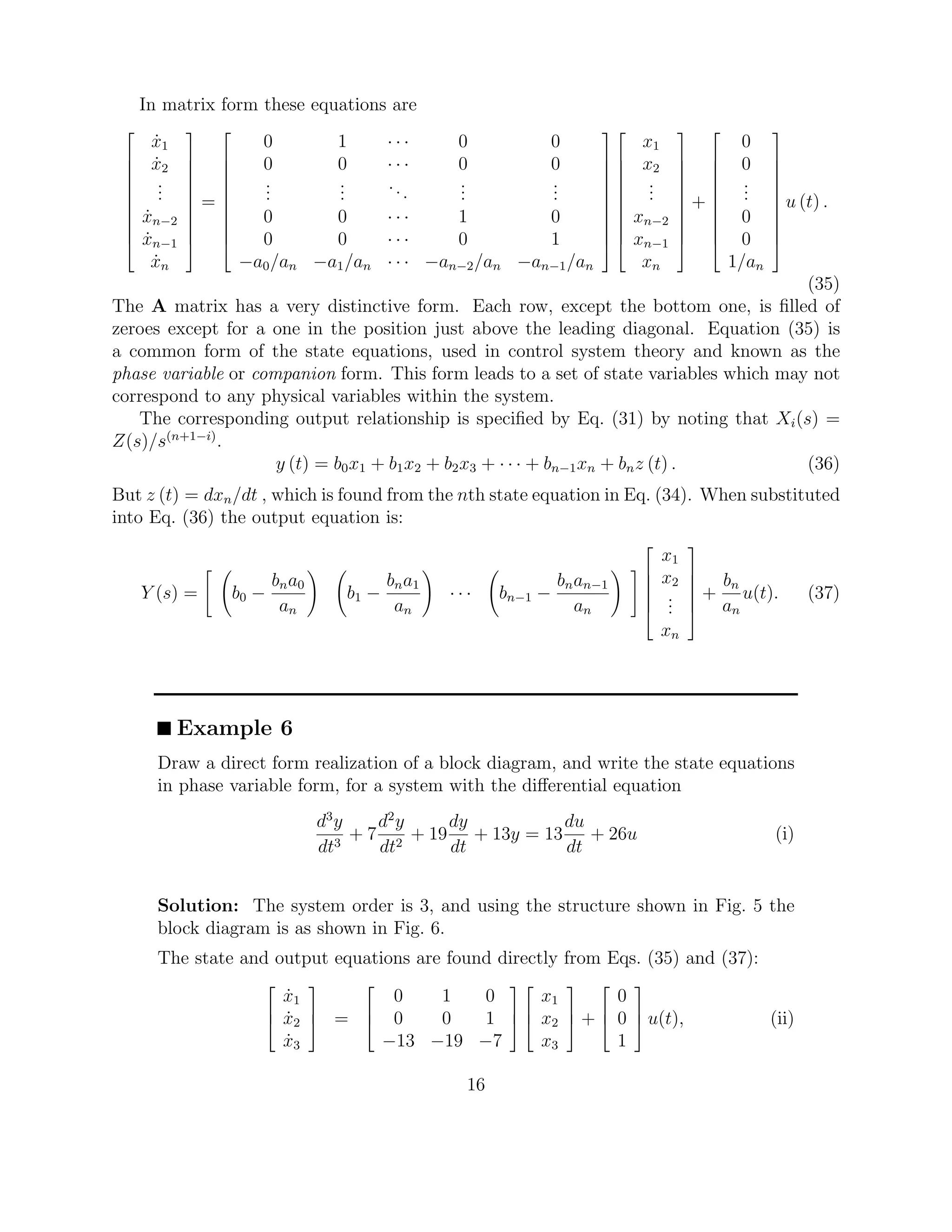
![Figure 6: Block diagram of the transfer operator of a third-order system found by a direct
realization.
y(t) = 26 13 0
x1
x2
x3
+ [0] u (t) . (iii)
5 The Matrix Transfer Function
For a multiple-input multiple-output system Eq. 22 is written in terms of the r component
input vector U(s)
X(s) = [sI − A]−1
BU(s) (38)
generating a set of n simultaneous linear equations, where the matrix is B is n × r. The m
component system output vector Y(s) may be found by substituting this solution for X(s)
into the output equation as in Eq. 25:
Y(s) = C [sI − A]−1
B {U(s)} + D {U(s)}
= C [sI − A]−1
B + D {U(s)} (39)
and expanding the inverse in terms of the determinant and the adjoint matrix
Y(s) =
C adj (sI − A) B + det [sI − A] D
det [sI − A]
U(s)
= H(s)U(s), (40)
where H(s) is defined to be the matrix transfer function relating the output vector Y(s) to
the input vector U(s):
H(s) =
(C adj (sI − A) B + det [sI − A] D)
det [sI − A]
(41)
17](https://image.slidesharecdn.com/statespace-190115163537/75/State-space-courses-17-2048.jpg)
![For a system with r inputs U1(s), . . . , Ur(s) and m outputs Y1(s), . . . , Ym(s), H(s) is a m×r
matrix whose elements are individual scalar transfer functions relating a given component
of the output Y(s) to a component of the input U(s). Expansion of Eq. 41 generates a set
of equations:
Y1(s)
Y2(s)
...
Ym(s)
=
H11(s) H12(s) · · · H1r(s)
H21(s) H22(s) · · · H2r(s)
...
...
...
...
Hm1(s) Hm2(s) · · · Hmr(s)
U1(s)
U2(s)
...
Ur(s)
(42)
where the ith component of the output vector Y(s) is:
Yi(s) = Hi1(s)U1(s) + Hi2(s)U2(s) + · · · + Hir(s)Us(s). (43)
The elemental transfer function Hij(s) is the scalar transfer function between the ith output
component and the jth input component. Equation 41 shows that all of the Hij(s) trans-
fer functions in H(s) have the same denominator factor det [sI − A], giving the important
result that all input-output differential equations for a system have the same characteristic
polynomial, or alternatively have the same coefficients on the left-hand side.
If the system has a single-input and a single-output, H(s) is a scalar, and the procedure
generates the input/output transfer operator directly.
18](https://image.slidesharecdn.com/statespace-190115163537/75/State-space-courses-18-2048.jpg)

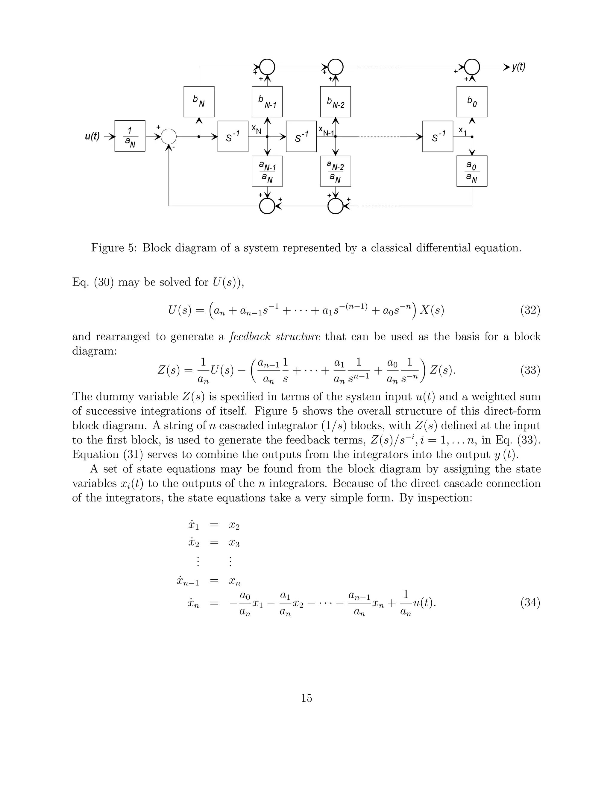
This document discusses state-space representation of linear time-invariant (LTI) systems. It defines system state, state equations, and output equations. The key points are: 1) State equations describe the dynamics of a system using first-order differential equations relating state variables. Output equations relate outputs to state variables and inputs. 2) For LTI systems, the state equations can be written in matrix form as dx/dt = Ax + Bu, and output equations as y = Cx + Du. 3) Block diagrams can be constructed from the state-space model, with integrators for each state variable and blocks representing the A, B, C, and D matrices.
Overview of classical control theory limitations. Introduction to modern control theory, emphasizing state-space representation for LTI systems.
Definition of system state using state variables to describe system dynamics. Concepts of energy storage elements and transformations of state variables.
Standard form of state equations, representation in vector form, and relation of derivatives to state variables and inputs in LTI systems.
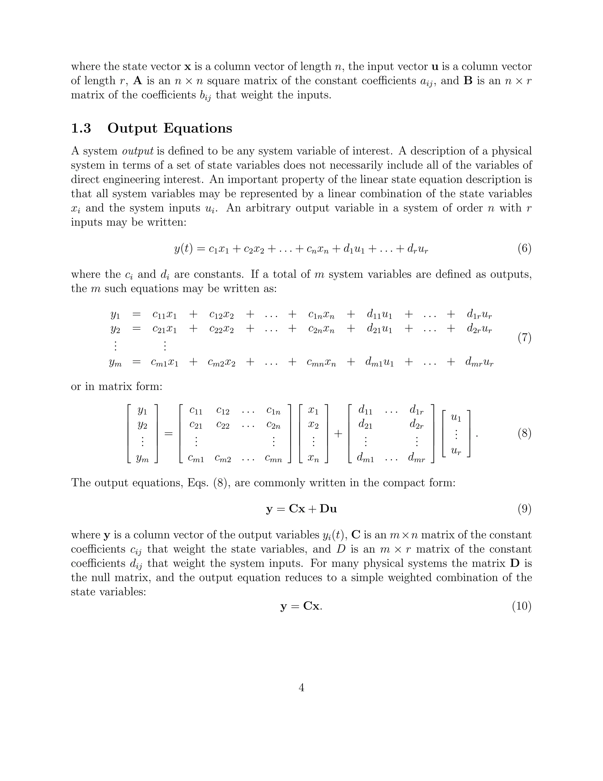
Definition of system output variables in terms of state variables and inputs. Relationship expressed using output equations and matrices C, D.
Procedure for constructing state-space models including determining system order and generating state equations from the system structure.
Construction of block diagram representation for linear systems using state equations, integrating system behavior visually.
Conversion from state-space representation to classical form using Laplace transforms to derive transfer functions and output relations.
Steps and examples of solving state equations to derive differential equations and transfer functions for dynamic systems.
Derivation of matrix transfer functions for multi-input multi-output systems, specifying relationships between outputs and inputs.