Download as PDF, PPTX


![PID controller and Lead-lag compensator
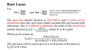
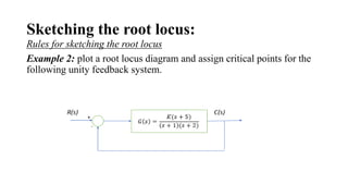
Example-1, [Norman Nise]
Given the system of figure below,
design a PD controller so that the
system can operate with a peak time
that is two thirds of that of
uncompensated system (0.3 sec) at
20% overshoot. The root locus of
uncompensated system is shown to
the right.](https://image.slidesharecdn.com/ch4-rootlocus-240426072734-4ef24b2d/85/Analysis-and-Design-of-Control-System-using-Root-Locus-27-320.jpg)
![PID controller and Lead-lag compensator
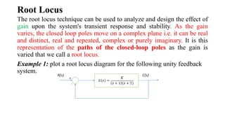
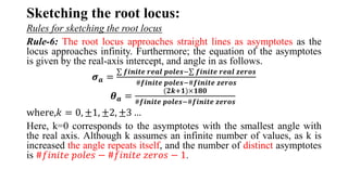
Example-2 [Norman Nise]
Upgrade the controller in example-1 to a PID controller that reduce the
steady state error to zero for a step input.](https://image.slidesharecdn.com/ch4-rootlocus-240426072734-4ef24b2d/85/Analysis-and-Design-of-Control-System-using-Root-Locus-28-320.jpg)

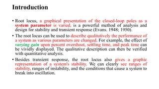
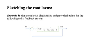
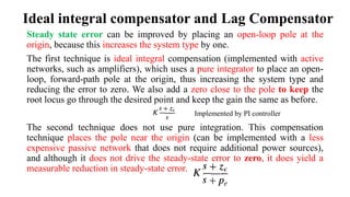
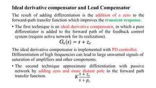
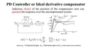
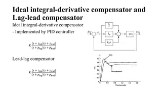
The document discusses the root locus method for analyzing and designing control systems, emphasizing its ability to illustrate system stability and transient response by varying gain. It outlines techniques and rules for sketching root loci, determining closed-loop poles, and identifying critical points, while also introducing compensation methods such as proportional, integral, and derivative control systems. Examples are provided to demonstrate practical applications of these concepts, illustrating how adjustments in system parameters impact performance outcomes.