Download to read offline


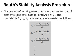

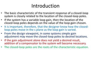
![Example 6–1 – p. 273 – Ogata V
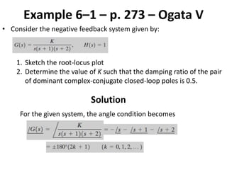
c) If -1 > s > -2, then:
Thus
(angle condition not satisfied)
d) If -2 > s > -∞, then:
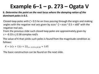
= 180°
Thus
-540° (angle condition satisfied)
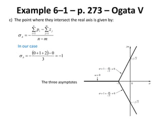
Thus, the portion of the real axis that lies on the root locus is given by:
]0,1[]2,[ S](https://image.slidesharecdn.com/classicalcontrol22-200916091122/85/Classical-control-2-2-39-320.jpg)

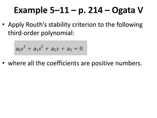
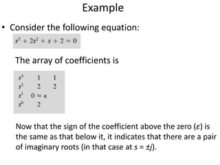
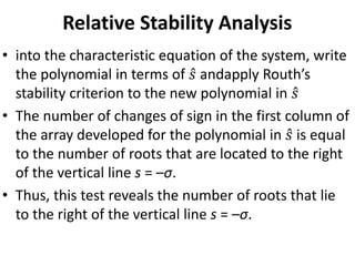
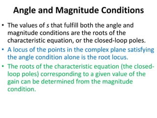
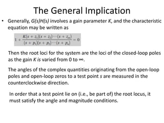
This document provides an overview of stability analysis in the frequency domain, including absolute stability, relative stability, Routh's stability criterion, and the root locus method. It defines absolute and relative stability and describes how Routh's stability criterion can be used to determine absolute stability by analyzing the signs of coefficients in the characteristic equation. The document also introduces the root locus method for analyzing how closed-loop poles move in the s-plane as the loop gain is varied.


![Roth_herwitz_stability_criterion-[1].pdf](https://cdn.slidesharecdn.com/ss_thumbnails/rothherwitzstabilitycriterion1-251026051926-6a7e967e-thumbnail.jpg?width=640&height=640&fit=bounds)


