This document discusses gradient descent optimization methods. It begins by explaining where gradient methods are used, such as in regression and machine learning problems. It then introduces several gradient descent algorithms - steepest descent, momentum, Nesterov's accelerated gradient, and others. It provides explanations of how each algorithm works. The document ends by performing benchmarks comparing the algorithms on MNIST data and a regression problem, finding that quasi-Newton and Adam methods tend to work best. In summary, it outlines common gradient descent optimization algorithms and compares their performance on sample problems.

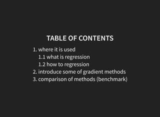
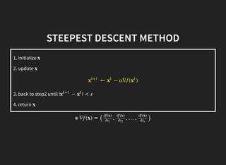
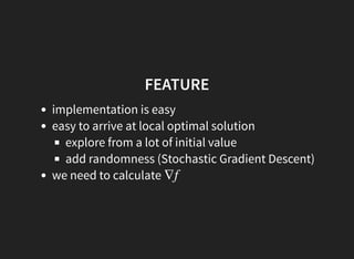
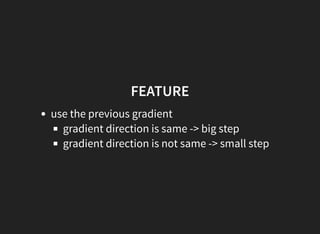
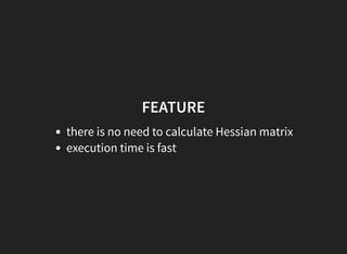
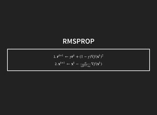
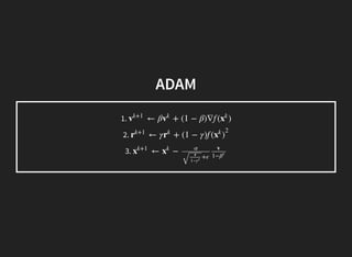
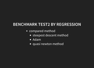
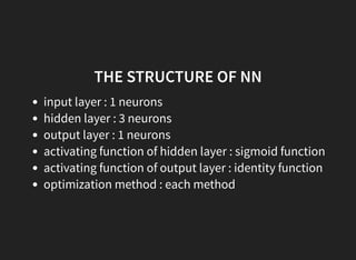
1. GRADIENT METHOD
2016/05/11
YAGI TAKAYUKI

2. TABLE OF CONTENTS
1. where it is used
1.1 what is regression
1.2 how to regression
2. introduce some of gradient methods
3. comparison of methods (benchmark)

3. Continue to fitting little by little
regression analysis

4. Continue to fitting little by little
regression analysis

5. Continue to fitting little by little
regression analysis

6. Continue to fitting little by little
regression analysis

7. Continue to fitting little by little
regression analysis

8. Continue to fitting little by little
regression analysis

9. Continue to fitting little by little
regression analysis

10. Continue to fitting little by little
regression analysis

11. Continue to fitting little by little
regression analysis

12. Continue to fitting little by little
regression analysis

13. Continue to fitting little by little
regression analysis

14. Continue to fitting little by little
regression analysis

15. HOW TO REGRESSION
reducing the error

16. THE MAIN IDEA OF REGRESSION
Minimization of the error function
it is called least squares method
E = ( − f ( )
1
2
∑n
i=1
yi xi )
2

17. SOLVE ??(x) = 0f
′
it is difficult to solve this equation
instead, we use optimization technique

18. WHERE IT IS USED ?
optimizaiton technique is used in optimization problem
machine learning is a kind of optimization problem

19. KIND OF OPTIMAIZATION ALGORITHM
using gradient
steepest descent method
newtons method
conjugate gradient method
not using gradient
genetic algorithm (GA)
simulated annealing (SA)
tabu search (TS)
I will introduce optimaization algorithm using a gradient

20. THERE ARE ALGORITHMS WHICH I
INTORODUCE
steepest descent method
momentum method
nesterovs accelerated gradient method
newton-raphson method
conjugate gradient method
quasi newton method
AdaGrad
RMSprop
AdaDelta
Adam

21. TODAY'S GOAL
introduce each algorithm simply
perform a benchmark test

22. CONFIGURATION
we think about minimization of we want to know
which takes minimum of
f (x) x
f (x)
is n-dimensional vector
is gradient of
is Hessian matrix
x
∇f f
H

23. STEEPEST DESCENT METHOD
Representative example of optimaization algorithm using a
gradient

24. STEEPEST DESCENT METHOD
1. initialize
2. update
3. back to step2 until
4. return
x
x
← − α∇f ( )x
k+1
x
k
x
k
| − | < εx
k+1
x
k
x
※ ∇f (x) =
( , , …,
)
∂f (x)
∂x1
∂f (x)
∂x2
∂f (x)
∂xn

25. STEEPEST DESCENT METHOD
1. initialize
2. update
3. back to step2 until
4. return
x
x
← − α∇f ( )x
k+1
x
k
x
k
| − | < εx
k+1
x
k
x
※ ∇f (x) =
( , , …,
)
∂f (x)
∂x1
∂f (x)
∂x2
∂f (x)
∂xn
later I will introduce only update expression

26. STEEPEST DESCENT METHOD
← − α∇f ( )x
k+1
x
k
x
k
is step sizeα

27. FEATURE
implementation is easy
easy to arrive at local optimal solution
explore from a lot of initial value
add randomness (Stochastic Gradient Descent)
we need to calculate ∇f

28. MOMENTUM METHOD
1.
2.
← β − α∇f ( )v
k+1
v
k
x
k
← +x
k+1
x
k
v
k+1
use previous gradient

29. NESTEROV'S ACCELERATED GRADIENT
METHOD
1.
2.
← β − α∇f ( + β )v
k+1
v
k
x
k
v
k
← +x
k+1
x
k
v
k+1
similar method of momentum method

30. FEATURE
use the previous gradient
gradient direction is same -> big step
gradient direction is not same -> small step

31. NEWTON METHOD
← −x
k+1
x
k ( )f
′
x
k
( )f
″
x
k
move to the extreme value of second-order approximate curve

32. NEWTON-RAPHSON METHOD
← − ∇f ( )x
k+1
x
k
H
−1
x
k
extend newton method to many variables

33. HESSIAN MATRIX

34. FEATURE
quadratic convergence (execution time is fast)
require inverse of hessian matrix（computational cost is
high）
preparing hessian matrix is difficult
need calcuration of inverse matrix（ ）( )n
3

35. CONJUGATE GRADIENT METHOD
1.
2.
3.
← −βk ( , ∇f ( ))m
k−1
H
k
x
k
( , )m
k−1
H
k
m
k−1
← ∇f ( ) +m
k
x
k
βk
m
k−1
← + αx
k+1
x
k
m
k
is inner product of(a, b) anda b

36. FEATURE
there is no need to calculate Hessian matrix
execution time is fast

37. QUASI NEWTON METHOD
is approximateH

38. ADAGRAD
1.
2.
← + ∇f (r
k+1
r
k
x
k
)
2
← − ∇f ( )x
k+1
x
k α
+εr
k+1
√
x
k

39. RMSPROP
1.
2.
← γ + (1 − γ)∇f (r
k+1
r
k
x
k
)
2
← − ∇f ( )x
k+1
x
k α
+εr
k+1
√
x
k

40. ADADELTA
1.
2.
3.
4.
← γ + (1 − γ)∇f (r
k+1
r
k
x
k
)
2
← ∇f ( )v
k+1
+εs
√
k
+εr√
k+1
x
k
← γ + (1 − γ)s
k+1
s
k
v
k+1
2
← −x
k+1
x
k
v
k+1

41. ADAM
1.
2.
3.
← β + (1 − β)∇f ( )v
k+1
v
k
x
k
← γ + (1 − γ)r
k+1
r
k
f ( )x
k
2
← −x
k+1
x
k α
+εr
1−γt
√
v
1−βt

42. BENCHMARK TEST1 BY MNIST
compared method
steepest descent method
momentum method
nesterovs accelerated gradient method
AdaGrad
RMSProp
AdaDelta
Adam
※ we can not use method using Hessian matrix

43. we can download data from
MNIST
here

44. NEURAL NETWORK
I used neural network model in this benchmark test

45. THE STRUCTURE OF NN
input layer : 784 neurons(28*28 dimension)
hidden layer : 100 neurons
output layer : 10 neurons (10 class)
activating function of hidden layer : sigmoid function
activating function of output layer : so max function
optimization method : each method

46. PARAMETER
I set parameters in each method by reference to
I select default parameters of each method
this website

47. RESULT1

48. RESULT1
AdaDelta, Adam, RMSProp showed good result
Note that I do not parameter tuning
in many cases, adam seems the best result

49. IS ADAM ALWAYS BEST APPROACH??
optimal method must be selected depending on the
problem
method using hessian matrix is very fast
it is better to chose, if you can choose

50. BENCHMARK TEST2 BY REGRESSION
compared method
steepest descent method
Adam
quasi newton method

51. THE STRUCTURE OF NN
input layer : 1 neurons
hidden layer : 3 neurons
output layer : 1 neurons
activating function of hidden layer : sigmoid function
activating function of output layer : identity function
optimization method : each method

52. RESULT2-1

53. RESULT2-2

54. RESULT2-3

55. RESULT2-4

56. RESULT2
quasi newton method showed best result
it is better to chose, if you can choose

57. CONCLUSION
we should choise method depending on the problem

58. thank you

59. REFERENCE