The document discusses Newton's backward interpolation formula, a method for estimating new data points within a range of known data. It outlines the history of interpolation, various types, and the implementation of the formula through examples and step-by-step calculations. Additionally, the document highlights the advantages and disadvantages of interpolation, as well as its applications in computer science, particularly in digital image processing and game development.


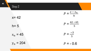
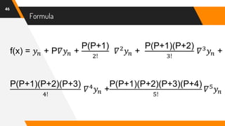
![Putting Values in Formula
47
f(42) = 204 + (-0.6)(-27) +
(−0.6)[(−0.6)+1]
2
(2)+
(−0.6)[(−0.6)+1][(−0.6)+2]
6
(0) +
(−0.6)[(−0.6)+1][(−0.6)+2][(−0.6)+3]
24
(8) +
(−0.6)[(−0.6)+1][(−0.6)+2][(−0.6)+3][(−0.6)+4]
120
(45)
= 204 + 16.2 + (−0.24) + 0 + (−0.26) + (−1.02)
f(42) = 216.68](https://image.slidesharecdn.com/nafinalpresentationf2018266065-copy-200701151927/85/Newton-s-Backward-Interpolation-Formula-with-Example-47-320.jpg)