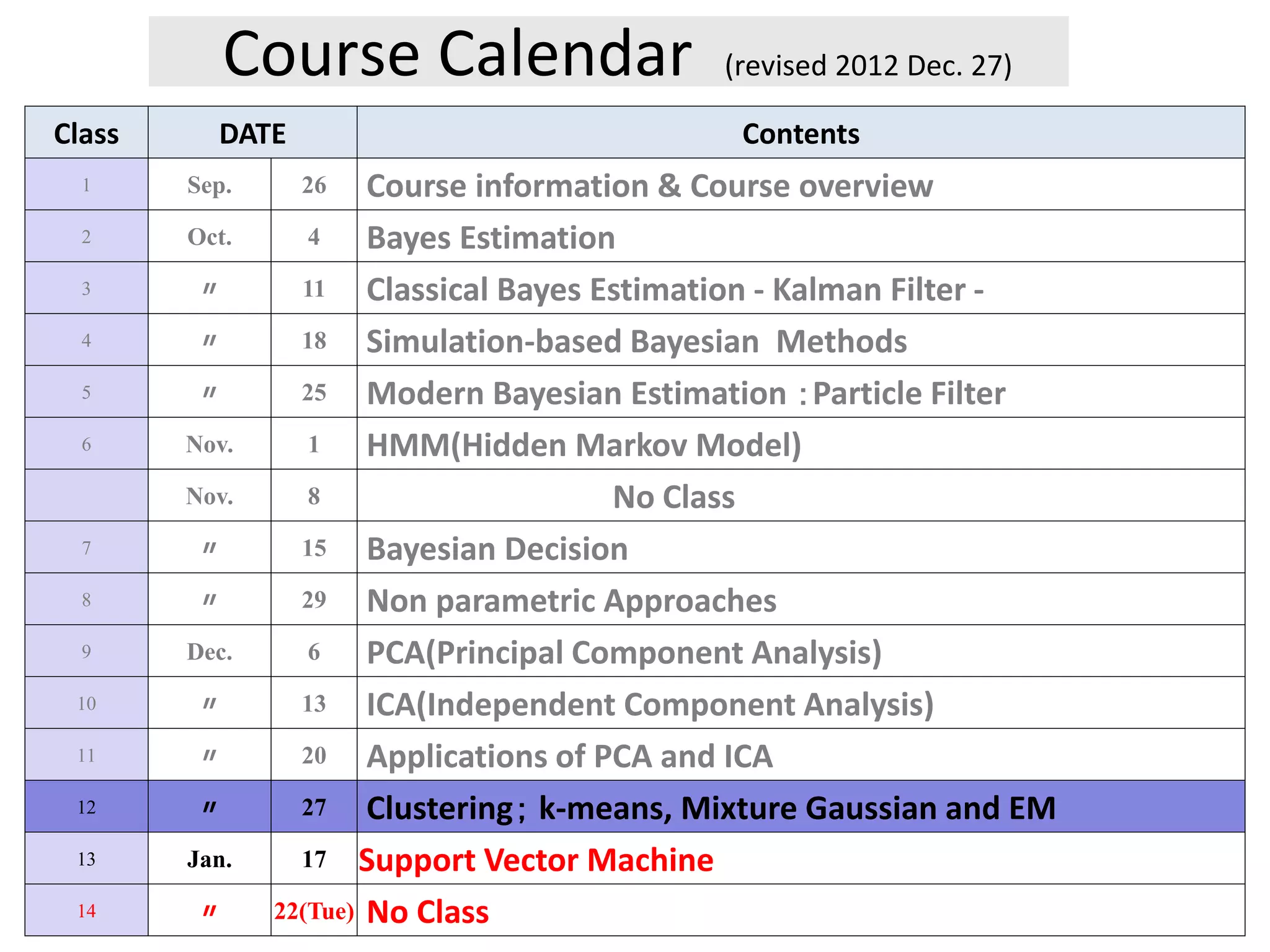
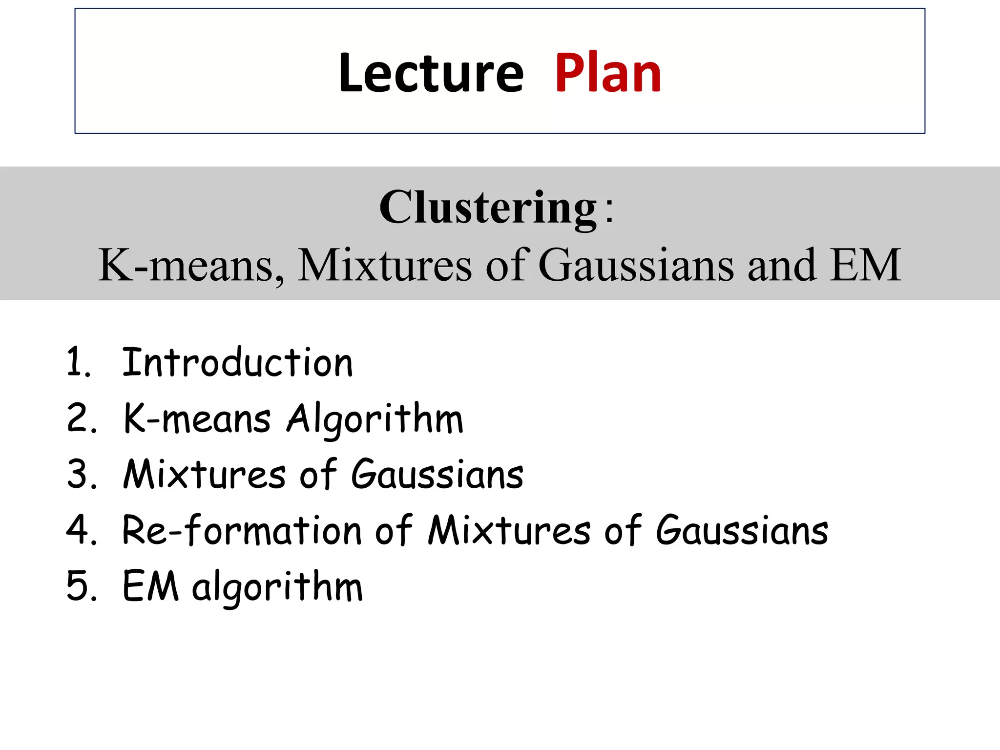
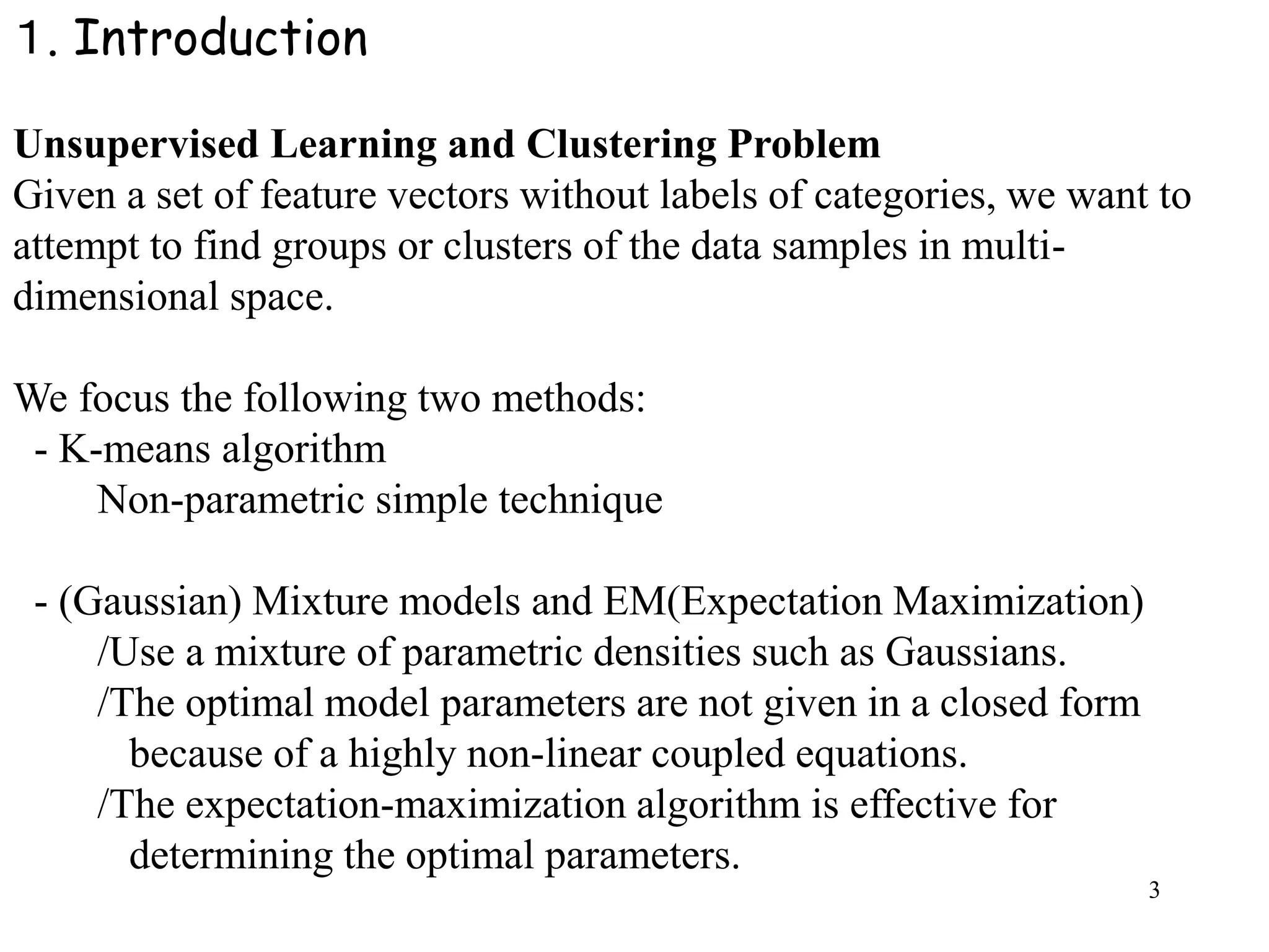
The document provides the course calendar and lecture plan for a machine learning course. The course calendar lists the class dates and topics to be covered from September to January, including Bayes estimation, Kalman filters, particle filters, hidden Markov models, Bayesian decision theory, principal component analysis, and clustering algorithms. The lecture plan focuses on clustering methods, including k-means clustering, mixtures of Gaussians models, and using the expectation-maximization (EM) algorithm to estimate the parameters of Gaussian mixture models.

1. Course Calendar (revised 2012 Dec. 27)
Class DATE Contents
1 Sep. 26 Course information & Course overview
2 Oct. 4 Bayes Estimation
3 〃 11 Classical Bayes Estimation - Kalman Filter -
4 〃 18 Simulation-based Bayesian Methods
5 〃 25 Modern Bayesian Estimation ：Particle Filter
6 Nov. 1 HMM(Hidden Markov Model)
Nov. 8 No Class
7 〃 15 Bayesian Decision
8 〃 29 Non parametric Approaches
9 Dec. 6 PCA(Principal Component Analysis)
10 〃 13 ICA(Independent Component Analysis)
11 〃 20 Applications of PCA and ICA
12 〃 27 Clustering； k-means, Mixture Gaussian and EM
13 Jan. 17 Support Vector Machine
14 〃 22(Tue) No Class

2. Lecture Plan
Clustering：
K-means, Mixtures of Gaussians and EM
1. Introduction
2. K-means Algorithm
3. Mixtures of Gaussians
4. Re-formation of Mixtures of Gaussians
5. EM algorithm

3. 3
１. Introduction
Unsupervised Learning and Clustering Problem
Given a set of feature vectors without labels of categories, we want to
attempt to find groups or clusters of the data samples in multi-
dimensional space.
We focus the following two methods:
- K-means algorithm
Non-parametric simple technique
- (Gaussian) Mixture models and EM(Expectation Maximization)
/Use a mixture of parametric densities such as Gaussians.
/The optimal model parameters are not given in a closed form
because of a highly non-linear coupled equations.
/The expectation-maximization algorithm is effective for
determining the optimal parameters.

4. 4
1 2
:D-dimensional random vector
N dataset of : X:={ , , , }
: A group of data points whose inter-distances are small
compared with the distances to the points outside of the cluster
N
Cluster
Prototy
x
x x x x
 
 
of cluster: 1
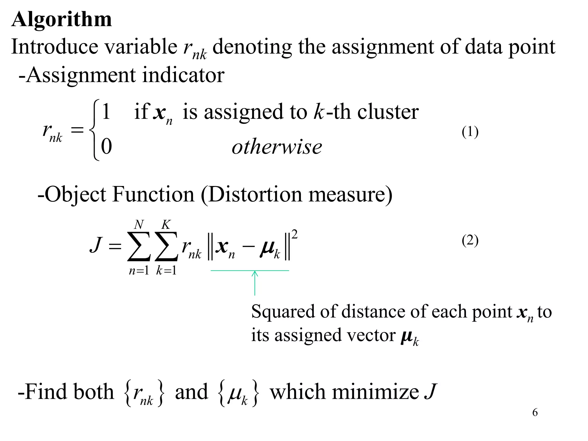
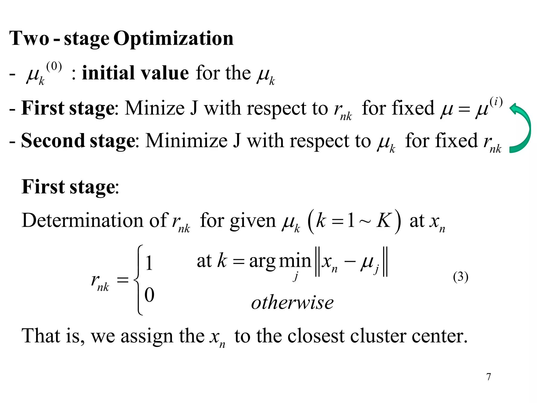
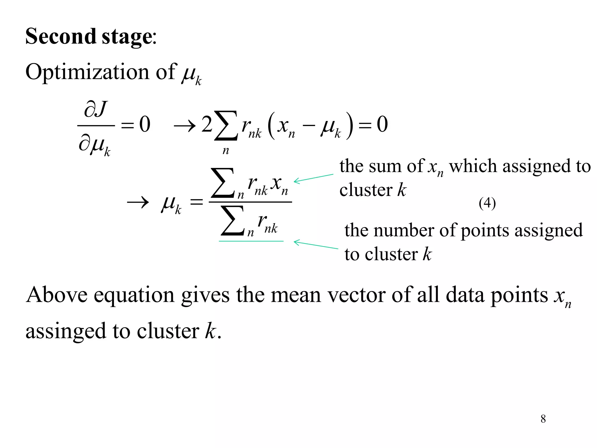
: Find a set of vectors , such that the sum of the squared
disstances of each point to its cvlosest vector is minimized.
k
k
k
k K
K



pe
Aim
2. K-means Algorithm
The K-means algorithm is a non-statistical approach of clustering of
data points in multi-dimensional feature space.
Problem: Partition the dataset into some number K of clusters
(K is known)
Fig. 1
1 [Bishop book[1] and its web site]

5. 5
Fig. 1
1 [Bishop book[1] and its web site]

6. 6
-Assignment indicator
1 if is assigned to -th cluster
0
n
nk
k
r
otherwise

 

x
Algorithm
Introduce variable rnk denoting the assignment of data point
2
1 1
-Object Function (Distortion measure)
N K
nk n k
n k
J r
 
  x 
Squared of distance of each point xn to
its assigned vector 𝝁k
   -Find both and which minimizenk kr J
(1)
(2)

7. 7
(0)
( )
- : for the
- : Minize J with respect to for fixed
- : Minimize J with respect to for fixed
k k
i
nk
k nk
r
r
 
 


Two - stage Optimization
initial value
First stage
Second stage
 
:
Determination of for given 1~ at
at argmin1
0
That is, we assign the to the closest cluster center.
nk k n
n j
j
nk
n
r k K x
k x
r
otherwise
x



  
 

First stage
(3)

8. 8
 
:
Optimization of
0 2 0
Above equation gives the mean vector of all data points
assinged to cluster .
k
nk n k
nk
nk nn
k
nkn
n
J
r x
r x
r
x
k





   

 



Second stage
the number of points assigned
to cluster k
the sum of xn which assigned to
cluster k
(4)

9. 9
Example 1 [Bishop book[1] and its web site]
Fig.2
(0)
1
(0)
2

10. Fig. 3 [1]
Application of k-means algorithm for color-based image
segmentation [Bishop book[1] and its web site]
K-means clustering applied to the color vectors of pixels in RGB
color-space

11. 11
   
1
[Mixture of Gaussians]
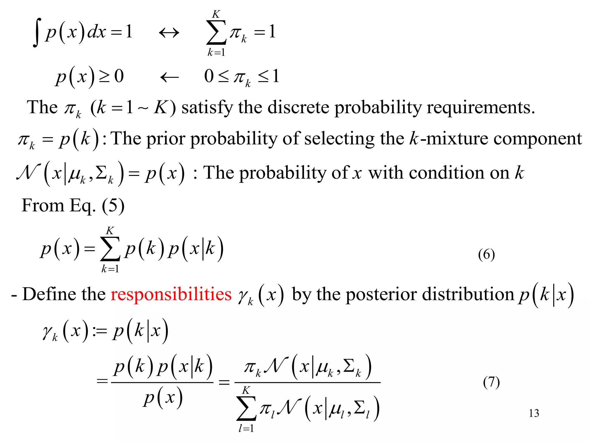
Conside a superposition of Gaussians (Normal distributions)
,
K
k k k
k
K
p x x 

 
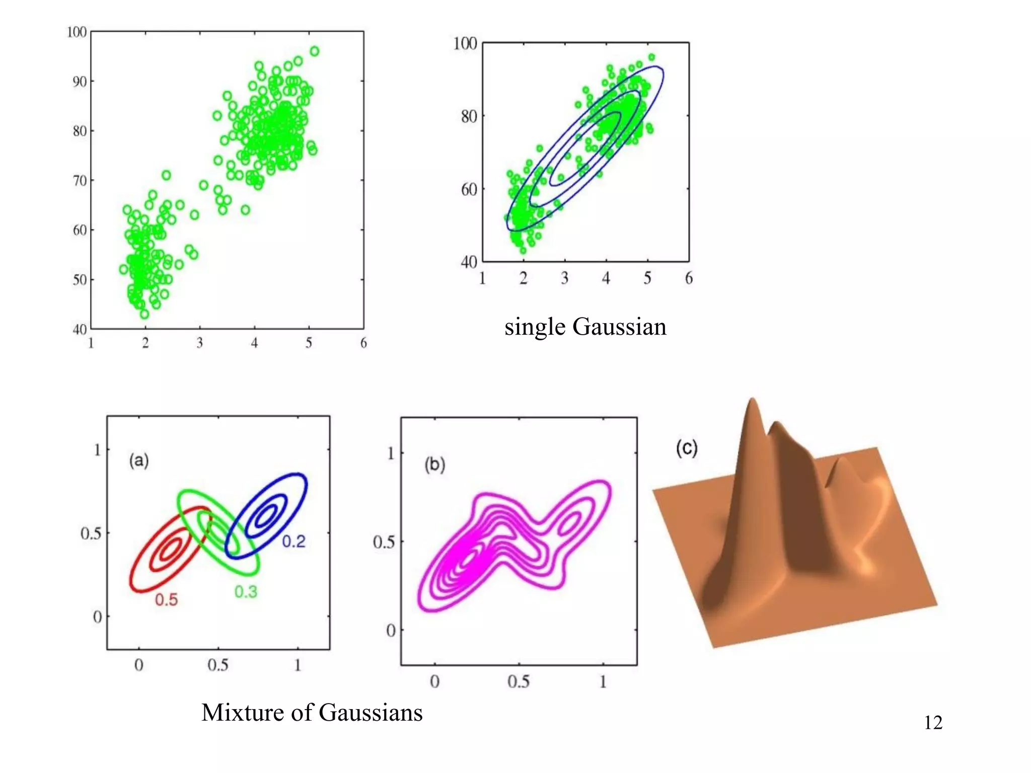
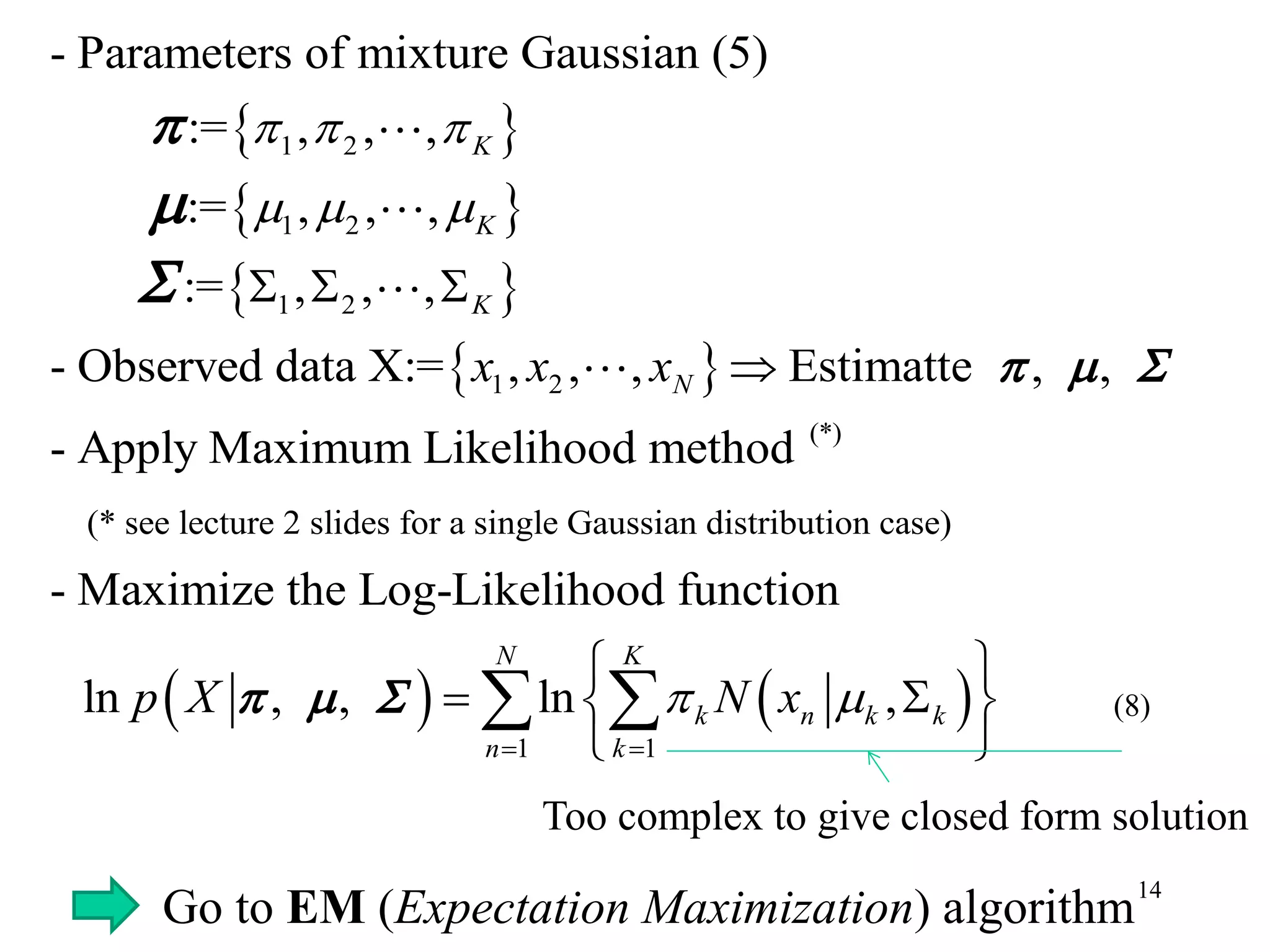
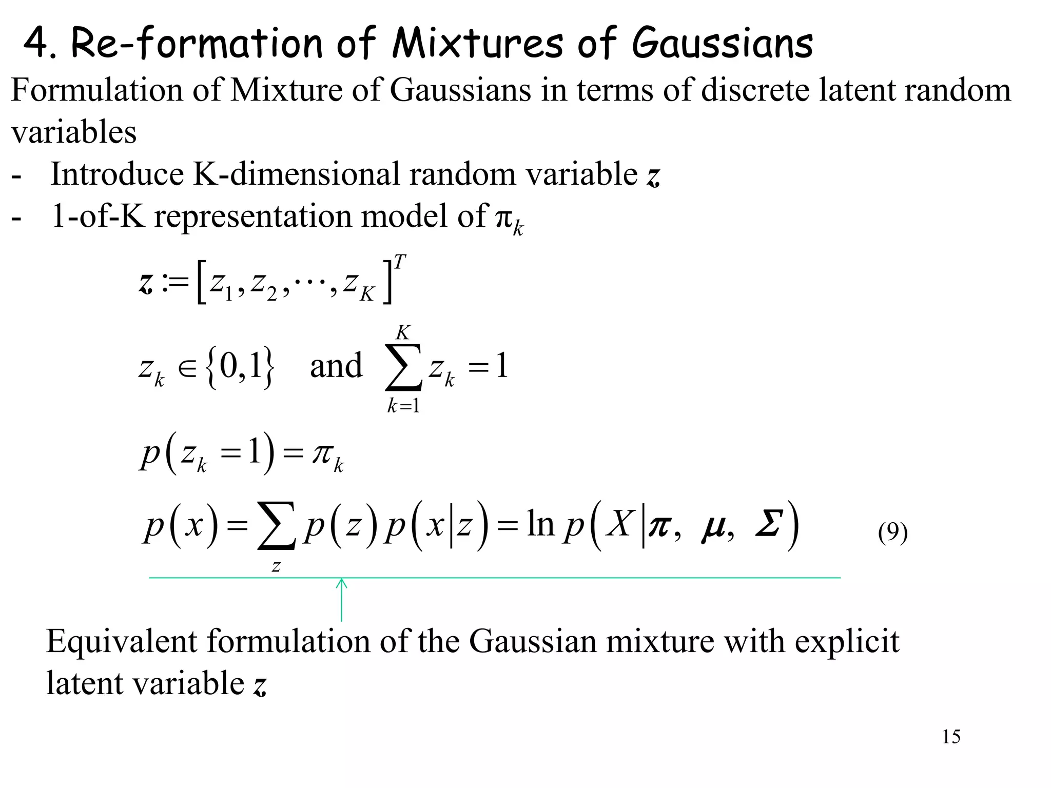
３. Mixtures of Gaussians
- Limitations of single Gaussian pdf model
Examples [Bishop[1]]
Single Gaussian model does not capture the multi-modes feature.
Fig 4
Mixture distribution approach: uses the linear combination of basic
distributions such as Gaussians
mixing coefficients mixture component
(5)
single Gaussian Mixture of Gaussians

12. 12
single Gaussian
Mixture of Gaussians

13. 13
 
 
 
   
1
1 1
0 0 1
The ( 1 ) satisfy the discrete probability requirements.
:The prior probability of selecting the -mixture component
,
K
k
k
k
k
k
k k
p x dx
p x
k K
p k k
x p x






  
   


 

     
   
   
   
 
 
 
1
responsibilit
: The probability of
i
with condition on
From Eq. (5)
- Define the by the posterior distributioe n
:
,
=
s
,
K
k
k
k
k k k
l l l
x k
p x p k p x k
x p k x
x p k x
p k p x k x
p x
x


 
 







1
K
l

(7)
(6)

14. 14
 
 
 
 
1 2
1 2
1 2
1 2
(*)
(* see lect
- Parameters of mixture Gaussian (5)
:= , , ,
:= , , ,
:= , , ,
- Observed data X:= , , , Estimatte , ,
- Apply Maximum Likelihood method
K
K
K
Nx x x
  
  
  
   



   
1 1
ure 2 slides for a single Gaussian distribution case)
- Maximize the Log-Likelihood function
ln , , ln ,
N K
k n k k
n k
p X N x 
 
 
  
 
   
Too complex to give closed form solution
Go to EM (Expectation Maximization) algorithm
(8)

15. 15
4. Re-formation of Mixtures of Gaussians
Formulation of Mixture of Gaussians in terms of discrete latent random
variables
- Introduce K-dimensional random variable z
- 1-of-K representation model of πk
 
 
 
1 2
1
: , , ,
0,1 and 1
1
T
K
K
k k
k
k k
z z z
z z
p z 


 
 

z
       ln , ,
z
p x p z p x z p X    
Equivalent formulation of the Gaussian mixture with explicit
latent variable z
(9)

16. 16
   
   
   
 
 1 1
- The conditional probability of for given
: 1
1 1 ,
1 1 ,
k k
k k k k k
K K
k k j j j
j j
z x
z p z x
p z p x z N x
p z p x z N x

 
 
 
 
  
 
   
The responsibility that component k
takes for explaining the observation x
The posterior probability for observed x
The prior probability of zk=1
 
   
1 2
1
- Modeling a data set X:= , , , using a mixture of Gaussians
Assuming , , are drawn independently from , ,
the Log-Likelihood function is given by Eq.()
N
N k k
x x x
x x p x  
(10)

17. 17
- With respect to and , the conditions that must be
satisfied at a maximum of the likelihood function
k k 
 
   
1 1
- Maximization of ln , , with respect to
subject to a constraint 1 is also solved.
- Solutions are given by
1
where :
k
kk
N N
k nk n k nk
n nk
k
p X
z x N z
N


  
 

 


 
  
   
 
1
The responsibility of with respect to -th cluster
1
where =Eq. (10) n
N
T
nk n k n k
nk
k
k
nk x k
z x x
N
N
N
z
  



  


5. EM Algorithm
 ln , ,
0, ,k k
p X
 


  

   (11)
(14)
(13)
(12)

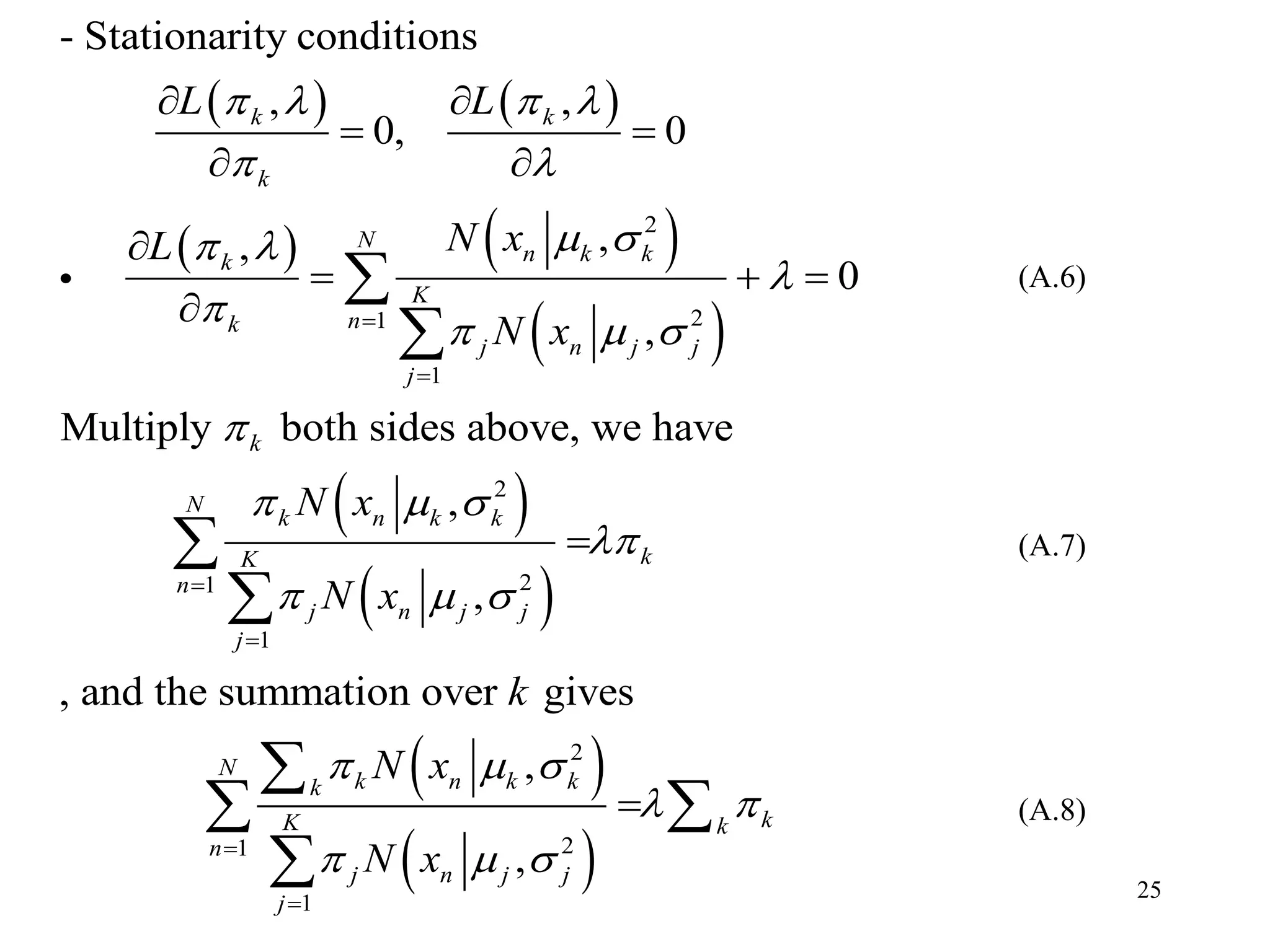
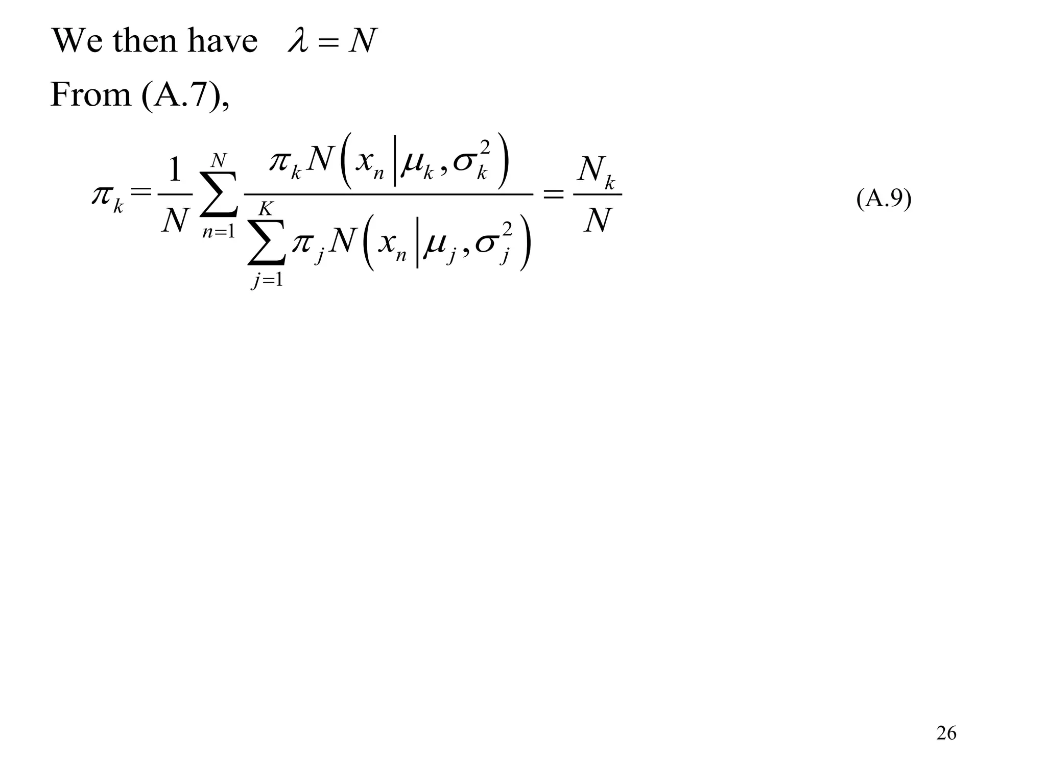
18. 18
 
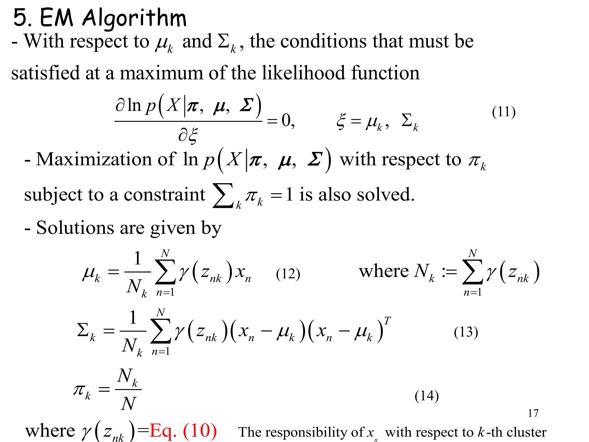
Three equations ()-() do not give solutions directly because
, contain unknowns , , and in complex ways.
[EM algorithm for Gaussian Mixture Mode]
Simple iterative scheme which altaernate the
nk kz N   
 
E (Expectation)
and M (Maximization) steps.
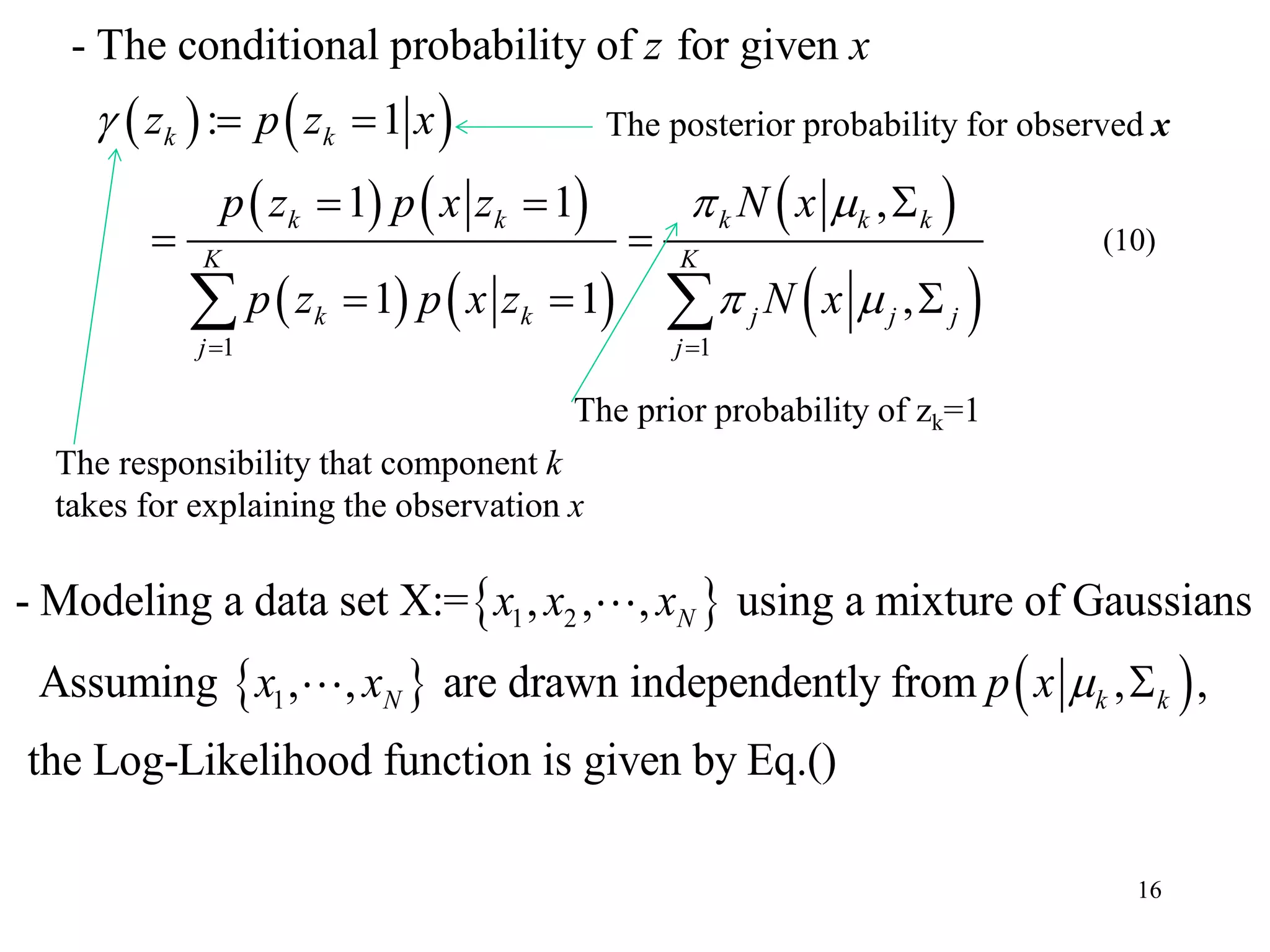
: Evaluate the posterior probabilities (responsibilities)
using the current parameters
: Re-estimate parameters , , a
nkz
 
E step
M step
 
 
nd using the
evaluated
Color illustration of in two-category case
nk
nk
z
z




19. 19
(0)
2
(0)
1

20. 20
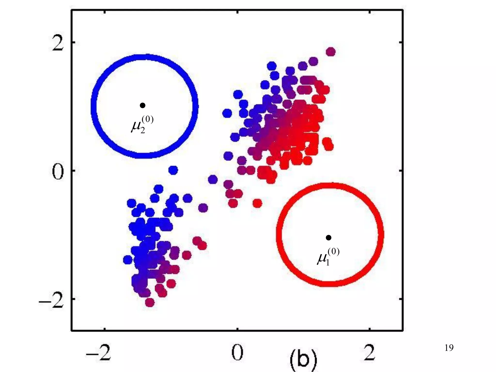
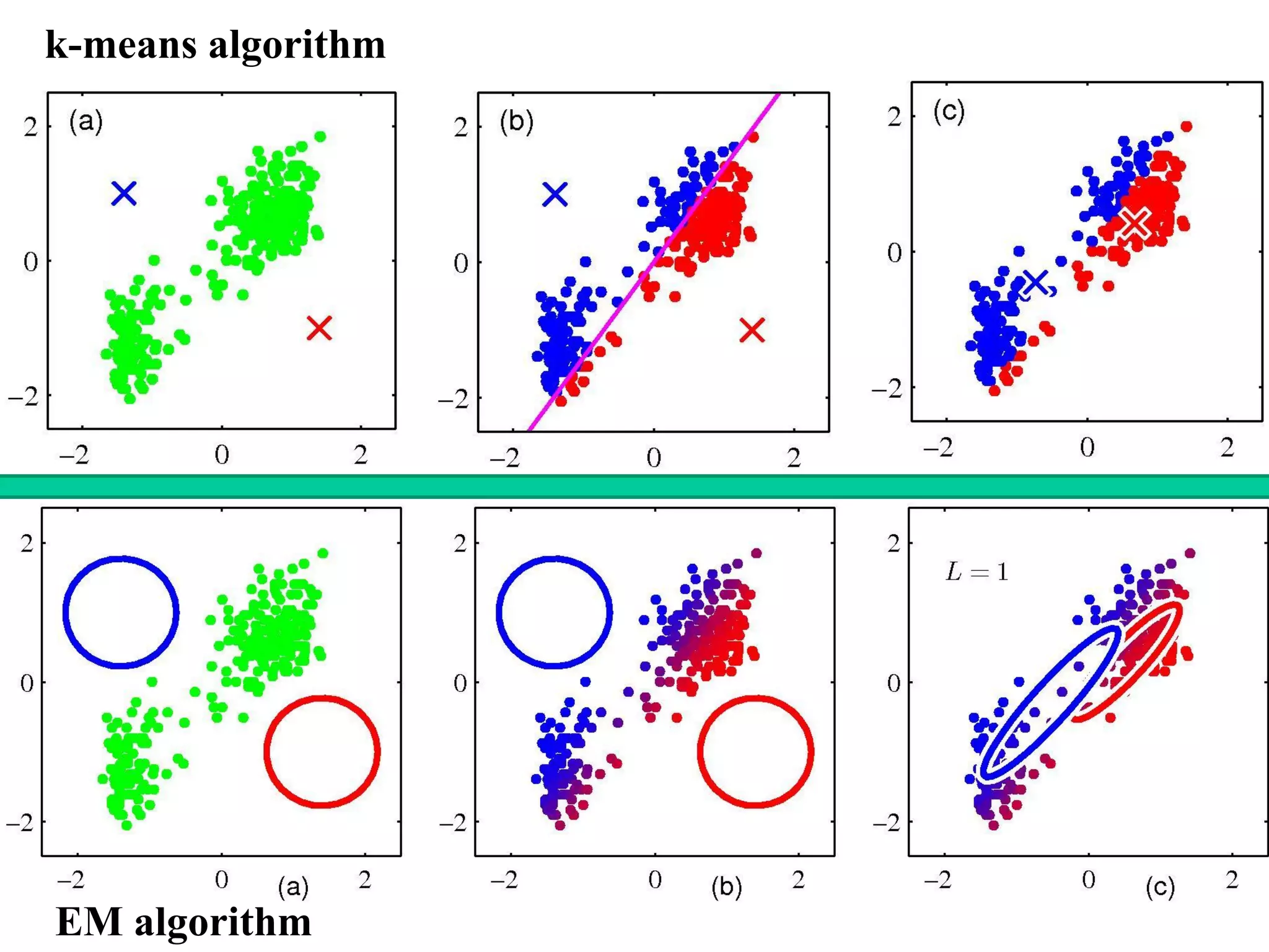
Example 2 EM algorithm [Bishop book[1] and its web site]
(0)
1
(0)
2

21. 21
k-means algorithm
EM algorithm

22. 22
References:
[1] C. M. Bishop, “Pattern Recognition and Machine Learning”,
Springer, 2006
[2] R.O. Duda, P.E. Hart, and D. G. Stork, “Pattern Classification”,
John Wiley & Sons, 2nd edition, 2004

23. 23
   
 
 
 
     
2
1 1
21
1
2
2 2
2
Proof of 1-dimensional case
ln , , ln ,
ln , , 0
,
- When
1
,
derives Eq.
,
,
1( 2)
n k k
n k k
N K
j n j j
n j
kN
K
n
j n j j
j
k
n k k n k
k k
N x
N x
p X N x
p X
N x
N x x
 


    

 

  
 
  



 


 
   
 





  


 
 


Appendix
(A.1)
(A.2)
(A.3)

24. 24
 
  
22
1
2
- When
Calculate and substitute it into Eq. (A.2)
derives
1
,
k
N
k nk n k
n
k
k
n
k
k
z x
N x
N
 

 
  


 



 
 
 
For the maximization problem of ln , , with respect
to subject to 1 , Lagrange multiplier method provides
an elegant solution.
- Introduce Lagragian function given by
, : ln ,
k kk
k
p X
L p X
 
 



  
    , 1kk
  
(A.4)
(A.5)

25. 25
   
   
 
 
 
2
21
1
2
21
1
- Stationarity conditions
, ,
0, 0
,,
0
,
Multiply both sides above, we have
,
,
, and the s
k k
k
N
n k kk
K
nk
j n j j
j
k
N
k n k k
kK
n
j n j j
j
L L
N xL
N x
N x
N x
   
 
  


  

  

  




 
 
 

  






 
 
2
21
1
ummation over gives
,
,
N
k n k kk
kK k
n
j n j j
j
k
N x
N x
  
 
  



 

(A.6)
(A.7)
(A.8)

26. 26
 
 
2
21
1
We then have
From (A.7),
,1
=
,
N
k n k k k
k K
n
j n j j
j
N
N x N
N N
N x

  

  




(A.9)