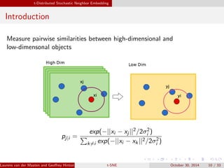
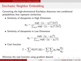
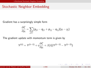
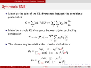
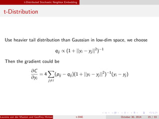
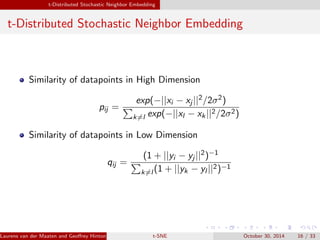
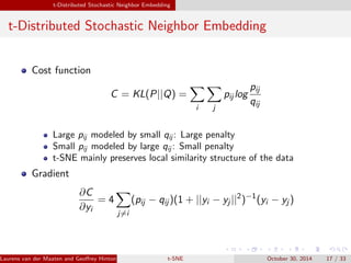
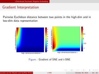
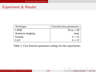
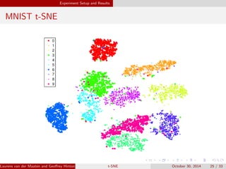
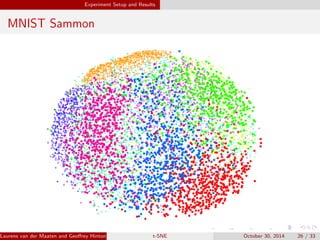
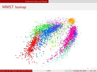
The document presents an overview of t-distributed Stochastic Neighbor Embedding (t-SNE), a technique for visualizing high-dimensional data in lower dimensions. It describes the methodology, including the preservation of local data similarities and the minimization of a cost function through gradient descent. Additionally, the document includes experimental results and resources for implementing t-SNE in various programming environments.

1. Visualizing Data using t-SNE
Laurens van der Maaten and Georey Hinton, JMLR 2008
Kevin Zhao
kevinzhaio@gmail.com
October 30, 2014
Laurens van der Maaten and Georey Hinton, JMLR 2008 (MCLta-bS)NE October 30, 2014 1 / 33

2. Overview
1 Overview
2 t-Distributed Stochastic Neighbor Embedding
3 Experiment Setup and Results
4 Code and Web Resources
Laurens van der Maaten and Georey Hinton, JMLR 2008 (MCLta-bS)NE October 30, 2014 2 / 33

3. Introduction
Overview
We are given a collection of N high-dimensional objects x1; :::xN
How can we get a feel for how these objects are arranged in the data
space?
Laurens van der Maaten and Georey Hinton, JMLR 2008 (MCLta-bS)NE October 30, 2014 3 / 33

4. Introduction
Principal Components Analysis
Laurens van der Maaten and Georey Hinton, JMLR 2008 (MCLta-bS)NE October 30, 2014 4 / 33

5. Introduction
Principal Components Analysis
Laurens van der Maaten and Georey Hinton, JMLR 2008 (MCLta-bS)NE October 30, 2014 5 / 33

6. Introduction
Swiss Roll
PCA is mainly concerned dimensionality, with preserving when large
pairwise distances in the map
Laurens van der Maaten and Georey Hinton, JMLR 2008 (MCLta-bS)NE October 30, 2014 6 / 33

7. t-Distributed Stochastic Neighbor Embedding
Introduction
Distance Perservation
Neighbor Perservation
Laurens van der Maaten and Georey Hinton, JMLR 2008 (MCLta-bS)NE October 30, 2014 7 / 33

8. t-Distributed Stochastic Neighbor Embedding
Introduction
Laurens van der Maaten and Georey Hinton, JMLR 2008 (MCLta-bS)NE October 30, 2014 8 / 33

9. t-Distributed Stochastic Neighbor Embedding
Introduction
Preserve the neighborhood
Laurens van der Maaten and Georey Hinton, JMLR 2008 (MCLta-bS)NE October 30, 2014 9 / 33

10. t-Distributed Stochastic Neighbor Embedding
Introduction
Measure pairwise similarities between high-dimensional and
low-dimensonal objects
pj ji =
exp(jjxi xj jj2=22
i ) P
k6=i exp(jjxi xk jj2=22
i )
Laurens van der Maaten and Georey Hinton, JMLR 2008 (MCLta-bS)NE October 30, 2014 10 / 33

11. t-Distributed Stochastic Neighbor Embedding
Stochastic Neighbor Embedding
Converting the high-dimensional Euclidean distances into conditional
probabilities that represent similarities
Similarity of datapoints in High Dimension
pj ji =
exp(jjxi xj jj2=22
i ) P
k6=i exp(jjxi xk jj2=22
i )
Similarity of datapoints in Low Dimension
qj ji =
exp(jjyi yj jj2 P )
k6=i exp(jjyi yk jj2)
Cost function
C =
X
i
KL(Pi jjQi ) =
X
i
X
j
pj ji log
pj ji
qj ji
Minimize the cost function using gradient descent
Laurens van der Maaten and Georey Hinton, JMLR 2008 (MCLta-bS)NE October 30, 2014 11 / 33

12. t-Distributed Stochastic Neighbor Embedding
Stochastic Neighbor Embedding
Gradient has a surprisingly simple form
@C
@yi
=
X
j6=i
(pj ji qj ji + pi jj qi jj )(yi yj )
The gradient update with momentum term is given by
Y (t) = Y (t1) +
@C
@yi
+

13. (t)(Y (t1) Y (t2))
Laurens van der Maaten and Georey Hinton, JMLR 2008 (MCLta-bS)NE October 30, 2014 12 / 33

14. t-Distributed Stochastic Neighbor Embedding
Symmetric SNE
Minimize the sum of the KL divergences between the conditional
probabilities
C =
X
i
KL(Pi jjQi ) =
X
i
X
j
pj ji log
pj ji
qj ji
Minimize a single KL divergence between a joint probability
distribution
C = KL(PjjQ) =
X
i
X
j6=i
pij log
pij
qij
The obvious way to rede

15. ne the pairwise similarities is
pij =
exp(jjxi xj jj2=22 P )
k6=l exp(jjxl xk jj2=22)
qij =
P exp(jjyi yj jj2)
k6=l exp(jjyl yk jj2)
Laurens van der Maaten and Georey Hinton, JMLR 2008 (MCLta-bS)NE October 30, 2014 13 / 33

16. t-Distributed Stochastic Neighbor Embedding
Symmetric SNE
Such that pij = pji ; qij = qji , the main advantage is simpli

17. ng the gradient
@C
@yi
= 2
X
j
(pij qij )(yi yj )
However, in practice we symmetrize (or average) the conditionals
pij =
pj ji + pi jj
2N
Set the bandwidth i such that the conditional has a

18. xed perplexity
(eective number of neighbors) Perp(Pi ) = 2H(Pi ), typical value is about 5
to 50
Laurens van der Maaten and Georey Hinton, JMLR 2008 (MCLta-bS)NE October 30, 2014 14 / 33

19. t-Distributed Stochastic Neighbor Embedding
t-Distribution
Use heavier tail distribution than Gaussian in low-dim space, we choose
qij / (1 + jjyi yj jj2)1
Then the gradient could be
@C
@yi
= 4
X
j6=i
(pij qij )(1 + jjyi yj jj2)1(yi yj )
Laurens van der Maaten and Georey Hinton, JMLR 2008 (MCLta-bS)NE October 30, 2014 15 / 33

20. t-Distributed Stochastic Neighbor Embedding
t-Distributed Stochastic Neighbor Embedding
Similarity of datapoints in High Dimension
pij =
exp(jjxi xj jj2=22 P )
k6=l exp(jjxl xk jj2=22)
Similarity of datapoints in Low Dimension
qij =
(1 + jjyi yj jj2)1
P
k6=l (1 + jjyk yl jj2)1
Laurens van der Maaten and Georey Hinton, JMLR 2008 (MCLta-bS)NE October 30, 2014 16 / 33

21. t-Distributed Stochastic Neighbor Embedding
t-Distributed Stochastic Neighbor Embedding
Cost function
C = KL(PjjQ) =
X
i
X
j
pij log
pij
qij
Large pij modeled by small qij : Large penalty
Small pij modeled by large qij : Small penalty
t-SNE mainly preserves local similarity structure of the data
Gradient
@C
@yi
= 4
X
j6=i
(pij qij )(1 + jjyi yj jj2)1(yi yj )
Laurens van der Maaten and Georey Hinton, JMLR 2008 (MCLta-bS)NE October 30, 2014 17 / 33

22. t-Distributed Stochastic Neighbor Embedding
Gradient Interpretation
Pairwise Euclidean distance between two points in the high-dim and in
low-dim data representation
Figure : Gradient of SNE and t-SNE
Laurens van der Maaten and Georey Hinton, JMLR 2008 (MCLta-bS)NE October 30, 2014 18 / 33

23. t-Distributed Stochastic Neighbor Embedding
Gradient Interpretation
We can interpret the t-SNE gradient as a simulation of an N-body system
@C
@yi
= 4
X
j6=i
(pij qij )(1 + jjyi yj jj2)1(yi yj )
Laurens van der Maaten and Georey Hinton, JMLR 2008 (MCLta-bS)NE October 30, 2014 19 / 33

24. t-Distributed Stochastic Neighbor Embedding
Gradient Interpretation
We can interpret the t-SNE gradient as a simulation of an N-body system
Displacement
(yi yj )
Laurens van der Maaten and Georey Hinton, JMLR 2008 (MCLta-bS)NE October 30, 2014 20 / 33

25. t-Distributed Stochastic Neighbor Embedding
Gradient Interpretation
We can interpret the t-SNE gradient as a simulation of an N-body system
Exertion / Compression
(pij qij )(1 + jjyi yj jj2)1
Laurens van der Maaten and Georey Hinton, JMLR 2008 (MCLta-bS)NE October 30, 2014 21 / 33

26. t-Distributed Stochastic Neighbor Embedding
Gradient Interpretation
We can interpret the t-SNE gradient as a simulation of an N-body system
N-Body, summation
@C
@yi
= 4
X
j6=i
(pij qij )(1 + jjyi yj jj2)1(yi yj )
Reduce Complexity from O(N2) to O(N log N) via Barnes Hut
(tree-based) algorithm
Laurens van der Maaten and Georey Hinton, JMLR 2008 (MCLta-bS)NE October 30, 2014 22 / 33

27. Experiment Setup and Results
Experiment Results
MNIST
Randomly selected 6,000 images
28 28 = 784 pixels
Olivetti faces
400 images (10 per individual)
92 112 = 10; 304 pixels
COIL-20
20 dierent objects and 72 equally spaced orientations, yielding a
total of 1,440 images
32 32 = 1024 pixels
Start by using PCA to reduce the dimensionality of the data to 30
Laurens van der Maaten and Georey Hinton, JMLR 2008 (MCLta-bS)NE October 30, 2014 23 / 33

28. Experiment Setup and Results
Experiment Results
Laurens van der Maaten and Georey Hinton, JMLR 2008 (MCLta-bS)NE October 30, 2014 24 / 33

29. Experiment Setup and Results
MNIST t-SNE
Laurens van der Maaten and Georey Hinton, JMLR 2008 (MCLta-bS)NE October 30, 2014 25 / 33

30. Experiment Setup and Results
MNIST Sammon
Laurens van der Maaten and Georey Hinton, JMLR 2008 (MCLta-bS)NE October 30, 2014 26 / 33

31. Experiment Setup and Results
MNIST Isomap
Laurens van der Maaten and Georey Hinton, JMLR 2008 (MCLta-bS)NE October 30, 2014 27 / 33

32. Experiment Setup and Results
MNIST LLE
Laurens van der Maaten and Georey Hinton, JMLR 2008 (MCLta-bS)NE October 30, 2014 28 / 33

33. Experiment Setup and Results
Olivetti faces
Laurens van der Maaten and Georey Hinton, JMLR 2008 (MCLta-bS)NE October 30, 2014 29 / 33