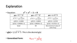
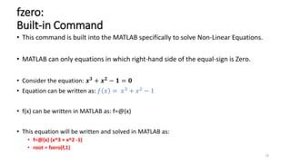
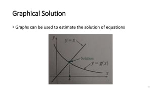
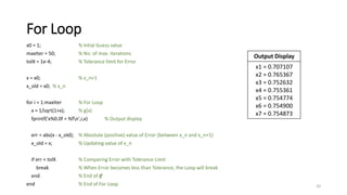
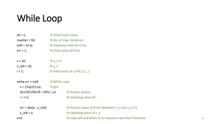
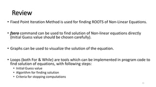
NUMERICAL METHODS LAB
(MT-202L)
Instructor: Engr. Ahmed Zaheer
Batch: 2k19 (5th Semester)
Session: Fall 2022
MED, HITEC University, Taxila
Fixed Point Iteration Method
2
OVERVIEW
3
What is it?
• A method for solving NON-LINEAR EQUATIONS
• Non-linear Equations (some examples):
• 4𝑥2 − 1 = 0
• 𝑥3 −𝑥2 +10 = 0
• 𝑦 = sin(𝑥)
• 𝑦 = log(𝑥)
4
Overview
• This is also called as Methods of successive substitution
• We solve f(x) = 0 in a different way
• Actually we solve x= g (x)
• Now we can write the above as x-g(x) = 0
• x-g(x) can now be called f(x)
xn+1 = g(xn)
• g(x) is also called the iteration function
5
Overview
• Plotting 2 graphs y=x & y=g(x)
• The point where the 2 plots intersect
is called the fixed point, is the solution
• The numerical value of x (solution) is
found by the iterative process
• The initial guess is a value of x which is
near the fixed point as the first guess and substitute in g(x)
6
Explanation
• Consider the equation: 𝒙𝟑 + 𝒙𝟐 − 𝟏 = 𝟎
• This equation can be written as: 𝑓 𝑥 = 𝑥3 + 𝑥2 − 1
• For x = 0, f(x) = -1
• For x = 1, f(x) = 1
• Solution (ROOT) of the equation will lie between -1 & 1 (b/c of changing sign)
• INITIAL GUESS: 𝑥0 = 0.5 (some other value could also be taken)
7
Explanation
• Equation: 𝒙𝟑 + 𝒙𝟐 − 𝟏 = 𝟎
• Equation can be rearranged as:
1. 𝑥 =
3
1 − 𝑥2 [ g(x) =
3
1 − 𝑥2 ]
2. 𝑥 = 1 − 𝑥3 [ g(x) = 1 − 𝑥3 ]
3. 𝑥 = 1/ 𝑥 + 1 [ g(x) = 1/ 𝑥 + 1 ]
• Which one of these “g(x)” is the correct one?
8
Explanation
• Equation: 𝒙𝟑 + 𝒙𝟐 − 𝟏 = 𝟎
• Which one of these “g(x)” is the correct one?
• CONDITION FOR CHECKING
|
𝒅[𝒈(𝒙)]
𝒅𝒙
| = |𝒈′
𝒙 | < 𝟏
The absolute value (i.e. positive value) of 1st differential of g(x) should be less
than 1 for the g(x) to be valid.
9
Explanation
• Equation: 𝒙𝟑
+ 𝒙𝟐
− 𝟏 = 𝟎
• g(x) = 1/ 𝑥 + 1 : This is the desired g(x)
• Generalized Form: 𝒙𝒏+𝟏 =
𝟏
𝟏+ 𝒙𝒏
10
g(x) =
𝟑
𝟏 − 𝐱𝟐 g(x) = 𝟏 − 𝐱𝟑 g(x) = 𝟏/ 𝐱 + 𝟏
𝑔′
𝑥 =
−2𝑥
3(1 − 𝑥2)2/3 𝑔′
𝑥 =
−3𝑥2
(1 − 𝑥3)1/2
𝑔′
𝑥 =
−1
2(𝑥+1)3/2
g’(0.5) = -0.4038 g’(0.5) = -0.8018 g’(0.5) = -0.2722
|g’(x)| = 0.4038 (< 1) |g’(x)| = 0.8018 (< 1) |g’(x)| = 0.2722 (< 1)
Good OK Best (minimum value of
g’(x) at 𝒙𝟎)
Explanation
• Equation: 𝒙𝟑 + 𝒙𝟐 − 𝟏 = 𝟎
• g(x) = 𝒙𝒏+𝟏 =
𝟏
𝟏+ 𝒙𝒏
• Root of Equation: 0.75488
11
i 𝒙𝒊 𝒙𝒊+𝟏 = 𝒈(𝒙)
0 0.5 0.81650
1 0.81650 0.74196
2 0.74196 0.75767
3 0.75767 0.75428
5 0.75428 0.75501
6 0.75501 0.75485
7 0.75485 0.75488
8 0.75488 0.75488
BUILT-IN FUNCTIONS
12
fzero:
Built-in Command
• This command is built into the MATLAB specifically to solve Non-Linear Equations.
• MATLAB can only equations in which right-hand side of the equal-sign is Zero.
• Consider the equation: 𝒙𝟑
+ 𝒙𝟐
− 𝟏 = 𝟎
• Equation can be written as: 𝑓 𝑥 = 𝑥3 + 𝑥2 − 1
• f(x) can be written in MATLAB as: f=@(x)
• This equation will be written and solved in MATLAB as:
• f=@(x) (x^3 + x^2 -1)
• root = fzero(f,1)
13
fzero:
Built-in Command
• Equation: 𝑓 𝑥 = 𝑥3 + 𝑥2 − 1
• This equation will be written and solved in MATLAB as:
• f=@(x) (x^3 + x^2 -1)
• fzero (f , 1) % This command will find the root of Function “ f ”, with Initial Guess value = 1
(Guess value can be changed to get the correct answer, or to get multiple roots)
• Output will be displayed as: ans = 0.7549
14
Graphical Solution
• Graphs can be used to estimate the solution of equations
15
Graphical Solution
• Equation: 𝒙𝟑 + 𝒙𝟐 − 𝟏 = 𝟎
• 𝑦 = 𝑥3 + 𝑥2 − 1
• 𝑦 = 𝑥
• Graphs can be drawn in MATLAB as:
x = -10:0.1:10;
% x is an array containing elements from -10 to +10, with incremental steps of 0.1
y1 = x.^3 + x.^2 - 1;
y2 = x;
plot(x,y1,x,y2) % For plotting multiple graphs using a single line of code
hold on
grid on
legend('y1','y2')
16
Graphical Solution
• Equation: 𝒙𝟑 + 𝒙𝟐 − 𝟏 = 𝟎
• 𝑦 = 𝑥3 + 𝑥2 − 1
• 𝑦 = 𝑥
• This graph can be zoomed for
better clarity.
• The point where the two curves
intersect, is the solution i.e.
the required
Root of the equation.
17
CODING THE ITERATION METHOD
18
Overview
• Iterative procedure for finding the root of an equation consists of 3
parts:
1. Initial Guess of solution
2. Algorithm for finding approximate solution
3. Criteria to Stop Computations
• Equation: 𝒙𝟑 + 𝒙𝟐 − 𝟏 = 𝟎
• g(x) = 𝒙𝒏+𝟏 =
𝟏
𝟏+ 𝒙𝒏
19
For Loop
x0 = 1; % Intial Guess value
maxIter = 50; % No. of max. iterations
tolX = 1e-4; % Tolerance limit for Error
x = x0; % x_n+1
x_old = x0; % x_n
for i = 1:maxIter % For Loop
x = 1/sqrt(1+x); % g(x)
fprintf('x%0.0f = %fn',i,x) % Output display
err = abs(x - x_old); % Absolute (positive) value of Error (between x_n and x_n+1)
x_old = x; % Updating value of x_n
if err < tolX % Comparing Error with Tolerance Limit
break % When Error becomes less than Tolerance, the Loop will break
end % End of If
end % End of For Loop 20
Output Display
x1 = 0.707107
x2 = 0.765367
x3 = 0.752632
x4 = 0.755361
x5 = 0.754774
x6 = 0.754900
x7 = 0.754873
While Loop
x0 = 1; % Intial Guess value
maxIter = 50; % No. of max. iterations
tolX = 1e-6; % Tolerance limit for Error
err = 1; % Intial value of Error
x = x0; % x_n+1
x_old = x0; % x_n
i = 1; % Intial value of i (i=0,1,2,...)
while err > tolX % While Loop
x = 1/sqrt(1+x); % g(x)
fprintf('x%0.0f = %fn',i,x) % Output display
i = i+1; % Updating value of i
err = abs(x - x_old); % Positive value of Error (between x_n and x_n+1)
x_old = x; % Updating value of x_n
end % Loop will end when Error becomes less than Tolerance 21
CONCLUSION
22
Review
• Fixed Point Iteration Method is used for finding ROOTS of Non-Linear Equations.
• fzero command can be used to find solution of Non-linear equations directly
(Initial Guess value should be chosen carefully).
• Graphs can be used to visualize the solution of the equation.
• Loops (both For & While) are tools which can be implemented in program code to
find solution of equations, with following steps:
• Initial Guess value
• Algorithm for finding solution
• Criteria for stopping computations
23
The End
• Thank you!
• Any Questions?
24

2. Fixed Point Iteration.pptx

  • 1.
    NUMERICAL METHODS LAB (MT-202L) Instructor:Engr. Ahmed Zaheer Batch: 2k19 (5th Semester) Session: Fall 2022 MED, HITEC University, Taxila
  • 2.
  • 3.
  • 4.
    What is it? •A method for solving NON-LINEAR EQUATIONS • Non-linear Equations (some examples): • 4𝑥2 − 1 = 0 • 𝑥3 −𝑥2 +10 = 0 • 𝑦 = sin(𝑥) • 𝑦 = log(𝑥) 4
  • 5.
    Overview • This isalso called as Methods of successive substitution • We solve f(x) = 0 in a different way • Actually we solve x= g (x) • Now we can write the above as x-g(x) = 0 • x-g(x) can now be called f(x) xn+1 = g(xn) • g(x) is also called the iteration function 5
  • 6.
    Overview • Plotting 2graphs y=x & y=g(x) • The point where the 2 plots intersect is called the fixed point, is the solution • The numerical value of x (solution) is found by the iterative process • The initial guess is a value of x which is near the fixed point as the first guess and substitute in g(x) 6
  • 7.
    Explanation • Consider theequation: 𝒙𝟑 + 𝒙𝟐 − 𝟏 = 𝟎 • This equation can be written as: 𝑓 𝑥 = 𝑥3 + 𝑥2 − 1 • For x = 0, f(x) = -1 • For x = 1, f(x) = 1 • Solution (ROOT) of the equation will lie between -1 & 1 (b/c of changing sign) • INITIAL GUESS: 𝑥0 = 0.5 (some other value could also be taken) 7
  • 8.
    Explanation • Equation: 𝒙𝟑+ 𝒙𝟐 − 𝟏 = 𝟎 • Equation can be rearranged as: 1. 𝑥 = 3 1 − 𝑥2 [ g(x) = 3 1 − 𝑥2 ] 2. 𝑥 = 1 − 𝑥3 [ g(x) = 1 − 𝑥3 ] 3. 𝑥 = 1/ 𝑥 + 1 [ g(x) = 1/ 𝑥 + 1 ] • Which one of these “g(x)” is the correct one? 8
  • 9.
    Explanation • Equation: 𝒙𝟑+ 𝒙𝟐 − 𝟏 = 𝟎 • Which one of these “g(x)” is the correct one? • CONDITION FOR CHECKING | 𝒅[𝒈(𝒙)] 𝒅𝒙 | = |𝒈′ 𝒙 | < 𝟏 The absolute value (i.e. positive value) of 1st differential of g(x) should be less than 1 for the g(x) to be valid. 9
  • 10.
    Explanation • Equation: 𝒙𝟑 +𝒙𝟐 − 𝟏 = 𝟎 • g(x) = 1/ 𝑥 + 1 : This is the desired g(x) • Generalized Form: 𝒙𝒏+𝟏 = 𝟏 𝟏+ 𝒙𝒏 10 g(x) = 𝟑 𝟏 − 𝐱𝟐 g(x) = 𝟏 − 𝐱𝟑 g(x) = 𝟏/ 𝐱 + 𝟏 𝑔′ 𝑥 = −2𝑥 3(1 − 𝑥2)2/3 𝑔′ 𝑥 = −3𝑥2 (1 − 𝑥3)1/2 𝑔′ 𝑥 = −1 2(𝑥+1)3/2 g’(0.5) = -0.4038 g’(0.5) = -0.8018 g’(0.5) = -0.2722 |g’(x)| = 0.4038 (< 1) |g’(x)| = 0.8018 (< 1) |g’(x)| = 0.2722 (< 1) Good OK Best (minimum value of g’(x) at 𝒙𝟎)
  • 11.
    Explanation • Equation: 𝒙𝟑+ 𝒙𝟐 − 𝟏 = 𝟎 • g(x) = 𝒙𝒏+𝟏 = 𝟏 𝟏+ 𝒙𝒏 • Root of Equation: 0.75488 11 i 𝒙𝒊 𝒙𝒊+𝟏 = 𝒈(𝒙) 0 0.5 0.81650 1 0.81650 0.74196 2 0.74196 0.75767 3 0.75767 0.75428 5 0.75428 0.75501 6 0.75501 0.75485 7 0.75485 0.75488 8 0.75488 0.75488
  • 12.
  • 13.
    fzero: Built-in Command • Thiscommand is built into the MATLAB specifically to solve Non-Linear Equations. • MATLAB can only equations in which right-hand side of the equal-sign is Zero. • Consider the equation: 𝒙𝟑 + 𝒙𝟐 − 𝟏 = 𝟎 • Equation can be written as: 𝑓 𝑥 = 𝑥3 + 𝑥2 − 1 • f(x) can be written in MATLAB as: f=@(x) • This equation will be written and solved in MATLAB as: • f=@(x) (x^3 + x^2 -1) • root = fzero(f,1) 13
  • 14.
    fzero: Built-in Command • Equation:𝑓 𝑥 = 𝑥3 + 𝑥2 − 1 • This equation will be written and solved in MATLAB as: • f=@(x) (x^3 + x^2 -1) • fzero (f , 1) % This command will find the root of Function “ f ”, with Initial Guess value = 1 (Guess value can be changed to get the correct answer, or to get multiple roots) • Output will be displayed as: ans = 0.7549 14
  • 15.
    Graphical Solution • Graphscan be used to estimate the solution of equations 15
  • 16.
    Graphical Solution • Equation:𝒙𝟑 + 𝒙𝟐 − 𝟏 = 𝟎 • 𝑦 = 𝑥3 + 𝑥2 − 1 • 𝑦 = 𝑥 • Graphs can be drawn in MATLAB as: x = -10:0.1:10; % x is an array containing elements from -10 to +10, with incremental steps of 0.1 y1 = x.^3 + x.^2 - 1; y2 = x; plot(x,y1,x,y2) % For plotting multiple graphs using a single line of code hold on grid on legend('y1','y2') 16
  • 17.
    Graphical Solution • Equation:𝒙𝟑 + 𝒙𝟐 − 𝟏 = 𝟎 • 𝑦 = 𝑥3 + 𝑥2 − 1 • 𝑦 = 𝑥 • This graph can be zoomed for better clarity. • The point where the two curves intersect, is the solution i.e. the required Root of the equation. 17
  • 18.
  • 19.
    Overview • Iterative procedurefor finding the root of an equation consists of 3 parts: 1. Initial Guess of solution 2. Algorithm for finding approximate solution 3. Criteria to Stop Computations • Equation: 𝒙𝟑 + 𝒙𝟐 − 𝟏 = 𝟎 • g(x) = 𝒙𝒏+𝟏 = 𝟏 𝟏+ 𝒙𝒏 19
  • 20.
    For Loop x0 =1; % Intial Guess value maxIter = 50; % No. of max. iterations tolX = 1e-4; % Tolerance limit for Error x = x0; % x_n+1 x_old = x0; % x_n for i = 1:maxIter % For Loop x = 1/sqrt(1+x); % g(x) fprintf('x%0.0f = %fn',i,x) % Output display err = abs(x - x_old); % Absolute (positive) value of Error (between x_n and x_n+1) x_old = x; % Updating value of x_n if err < tolX % Comparing Error with Tolerance Limit break % When Error becomes less than Tolerance, the Loop will break end % End of If end % End of For Loop 20 Output Display x1 = 0.707107 x2 = 0.765367 x3 = 0.752632 x4 = 0.755361 x5 = 0.754774 x6 = 0.754900 x7 = 0.754873
  • 21.
    While Loop x0 =1; % Intial Guess value maxIter = 50; % No. of max. iterations tolX = 1e-6; % Tolerance limit for Error err = 1; % Intial value of Error x = x0; % x_n+1 x_old = x0; % x_n i = 1; % Intial value of i (i=0,1,2,...) while err > tolX % While Loop x = 1/sqrt(1+x); % g(x) fprintf('x%0.0f = %fn',i,x) % Output display i = i+1; % Updating value of i err = abs(x - x_old); % Positive value of Error (between x_n and x_n+1) x_old = x; % Updating value of x_n end % Loop will end when Error becomes less than Tolerance 21
  • 22.
  • 23.
    Review • Fixed PointIteration Method is used for finding ROOTS of Non-Linear Equations. • fzero command can be used to find solution of Non-linear equations directly (Initial Guess value should be chosen carefully). • Graphs can be used to visualize the solution of the equation. • Loops (both For & While) are tools which can be implemented in program code to find solution of equations, with following steps: • Initial Guess value • Algorithm for finding solution • Criteria for stopping computations 23
  • 24.
    The End • Thankyou! • Any Questions? 24