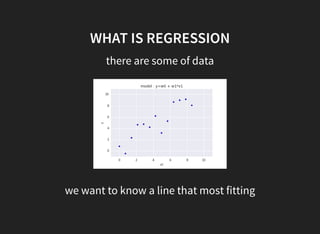
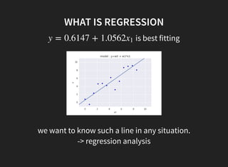
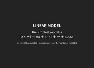
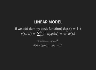
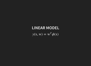
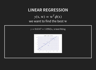
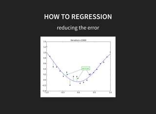
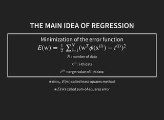
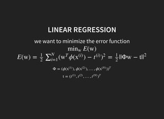
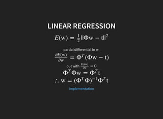
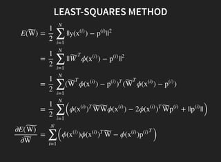
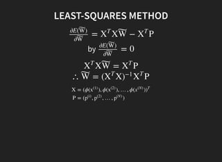
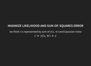
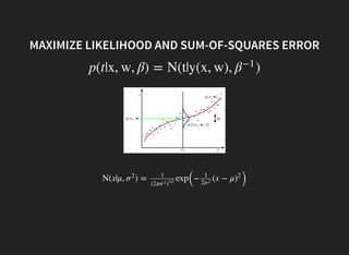
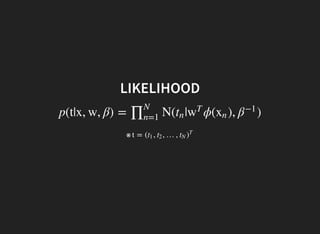
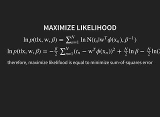
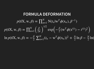
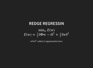
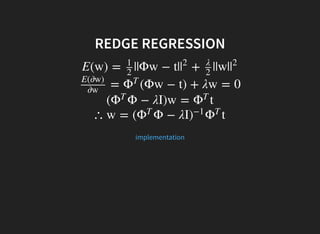
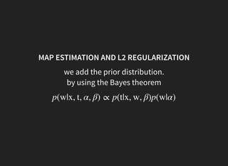
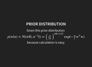
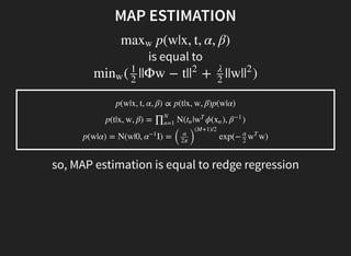
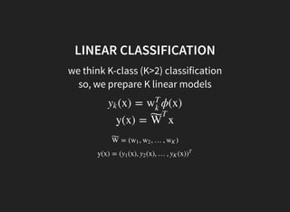
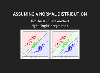
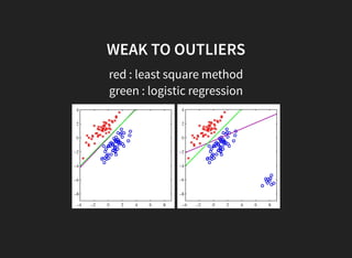
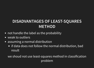
I introduced some key concepts in linear regression models: 1. Linear regression aims to fit a linear function to data to minimize error. 2. Maximum likelihood estimation is equivalent to least squares regression. 3. MAP estimation with a Gaussian prior is equivalent to ridge regression. 4. Linear classification models predict class probabilities using multiple linear functions. 5. The least squares method for classification has disadvantages like being sensitive to outliers.

1. LINEAR MODEL
2016/06/08
Yagi Takayuki

2. REFERENCE
Pattern Recognition and Machine Learning (PRML)
chapter3,4

3. TABLE OF CONTENTS
1. linear regression
1.1. what is regression
1.2. linear regression
1.3. ridge regression
1.4. lasso regression
1.5. generalization
1.6. maximum likelihood estimation
1.7. MAP estimation
2. linear classification
2.1. multi-class classification
2.2. disadvandages of least squares method

4. we want to know a line that most fitting
WHAT IS REGRESSION
there are some of data

5. we want to know such a line in any situation.
-> regression analysis
WHAT IS REGRESSION
is best fittingy = 0.6147 + 1.0562x1

6. NOTATION
: scalarx, w, t
: vectorx, w, t
: matrixX, W, T

7. LINEAR MODEL
the simplest model is
y(x, w) = + + ⋯ +w0 w1 x1 wD xD
: weight parameteswi : variablesxi : the number of variablesD

8. FEATURE
linear with respect to
linear with respect to
model is too simple (poor expressive power)
w
x

9. EXTEND THE MODEL
add linear combination of the non-linear function
y(x, w) = + (x)w0 ∑M−1
j=1
wj ϕj
is number of basis functionsM − 1
called basis function(x)ϕj
called bias parameterw0

10. LINEAR MODEL
if we add dummy basis function( )(x) = 1ϕ0
y(x, w) = (x) = ϕ(x)∑M−1
j=0
wj ϕj w
T
w = ( , …,w0 wM−1 )
T
ϕ(x) = ( (x), …, (x)ϕ0 ϕM−1 )
T

11. BASIS FUNCTION
there are various choices for the basis function
polynomial basis
gaussian basis
logistic sigmoid basis

12. POLYNOMIAL BASIS
(x) =ϕj x
j

13. GAUSSIAN BASIS
(x) = exp
(
− )
ϕj
(x−μj
)
2
2s
2

14. LOGISTIC SIGMOID BASIS
(x) = σ( )
ϕj
x−μj
s
σ(a) =
1
1+exp (−a)

15. LINEAR MODEL
y(x, w) = ϕ(x)w
T

16. FEATURE
linear with respect to
non-linear with respect to
we can choose a favorite basis
w
x

17. LINEAR REGRESSION
we want to find the best
y(x, w) = ϕ(x)w
T
w
is best fittingy = 0.6147 + 1.0562x1

18. HOW TO REGRESSION
reducing the error

19. THE MAIN IDEA OF REGRESSION
Minimization of the error function
: number of data
: i-th data
: target value of i-th data
E(w) = ( ϕ( ) −1
2
∑N
i=1
w
T
x
(i)
t
(i)
)
2
N
x
(i)
t
(i)
※ called least squares method
※
E(w)minw
called sum-of-squares errorE(w)

20. LINEAR REGRESSION
we want to minimize the error function
E(w)minw
E(w) = ( ϕ( ) − = ||Φw − t|
1
2
∑N
i=1
w
T
x
(i)
t
(i)
)
2 1
2
|
2
Φ = (ϕ( ), ϕ( ), …, ϕ( )x
(1)
x
(2)
x
(N)
)
T
t = ( , , …,t
(1)
t
(2)
t
(N)
)
T

21. LINEAR REGRESSION
E(w) = ||Φw − t|
1
2
|
2
partial differential in w
= (Φw − t)
∂E(w)
∂w
Φ
T
put with = 0
E(∂w)
∂w
Φw = tΦ
T
Φ
T
∴ w = ( Φ tΦ
T
)
−1
Φ
T
implementation

22. REDGE REGRESSIN
E(w)minw
E(w) = ||Φw − t| + ||w|
1
2
|
2 λ
2
|
2
※ called L2 regularization term||w||
2

23. REDGE REGRESSION
E(w) = ||Φw − t| + ||w|
1
2
|
2 λ
2
|
2
= (Φw − t) + λw = 0
E(∂w)
∂w
Φ
T
( Φ − λI)w = tΦ
T
Φ
T
∴ w = ( Φ − λI tΦ
T
)
−1
Φ
T
implementation

24. LASSO REGRESSION
E(w) = ||Φw − t| + |w|
1
2
|
2 λ
2
∑M−1
j=1
※ called L1 regularization term|w|

25. LASSO REGRESSION
not be solved analytically (nondifferentiable)
solved by coordinate descent
perform variable selection(some of the parameters to 0)
implementation

26. GENERALIZATION
general of the redge and lasso
E(w) = ||Φt − t| + |w
1
2
|
2 λ
2
∑M−1
j=1
|
q

27. RE-EXPRESSION
is equal to
s.t.
(
||Φw − t| + |w
)
minw
1
2
|
2 λ
2
∑M
j=1
|
q
||Φw − t|minw
1
2
|
2
| ≤ η∑M
j=1
wj |
q
※ is calculated from lagrange multiplier methodη

28. IMAGE
le : redge regression
right : lasso regression

29. PROOF
s.t.( ϕ( ) −minw
1
2
∑N
i=1
w
T
x
(i)
t
(i)
)
2
| ≤ η∑M
j=1
wj |
q
by using the Lagrange multiplier method
L(w, λ) = ( ϕ( ) − + ( | − η)
1
2
∑N
i=1
w
T
x
(i)
t
(i)
)
2 λ
2
∑M
j=1
wj |
q
by using KKT conditions
= | − η∂L(w,λ)
∂λ ∑M
j=1
wj |
q
∴ | = η∑M
j=1
w
∗
j
|
q

30. MAXIMIZE LIKELIHOOD AND SUM-OF-SQUARES ERROR
we think is represented by sum of and Gaussian noiset y(x, w)
t = y(x, w) + ε

31. MAXIMIZE LIKELIHOOD AND SUM-OF-SQUARES ERROR
p(t|x, w, β) = N(t|y(x, w), )β−1
N(x|μ, ) = exp
(
− (x − μ )
σ2 1
(2πσ2
)
1/2
1
2σ2
)
2

32. LIKELIHOOD
p(t|x, w, β) = N( | ϕ( ), )∏N
n=1
tn w
T
xn β−1
※ t = ( , , …,t1 t2 tN )
T

33. MAXIMIZE LIKELIHOOD
ln p(t|x, w, β) = ln N( | ϕ( ), )∑N
n=1
tn w
T
xn β−1
ln p(t|x, w, β) = − ( − ϕ( ) + ln β − ln(2
β
2
∑N
n=1
tn w
T
xn )
2 N
2
N
2
therefore, maximize likelifood is equal to minimize sum-of-squares error

34. FORMULA DEFORMATION
p(t|X, w, β) = N( | ϕ( ), )∏N
n=1
tn w
T
xn β−1
p(t|X, w, β) =
(
exp
(
− ( ϕ( ) − )
∏N
n=1
β
2π )
1/2
β
2
w
T
x
(i)
t
(i)
)
2
ln p(t|X, w, β) = − ( − ϕ( ) + ln β − ln(
β
2
∑N
n=1
tn w
T
xn )
2 N
2
N
2

35. MAP ESTIMATION AND L2 REGULARIZATION
we add the prior distribution.
by using the Bayes theorem
p(w|x, t, α, β) ∝ p(t|x, w, β)p(w|α)

36. PRIOR DISTRIBUTION
Given this prior distribution
because calculation is easy.
p(w|α) = N(w|0, I) =
(
exp(− w)α−1 α
2π )
(M+1)/2
α
2
w
T

37. MAP ESTIMATION
is equal to
p(w|x, t, α, β)maxw
( ||Φw − t| + ||w| )minw
1
2
|
2 λ
2
|
2
p(w|x, t, α, β) ∝ p(t|x, w, β)p(w|α)
p(t|x, w, β) = N( | ϕ( ), )∏N
n=1
tn w
T
xn β−1
p(w|α) = N(w|0, I) =
(
exp(− w)α−1 α
2π )
(M+1)/2
α
2
w
T
so, MAP estimation is equal to redge regression

38. FORMULA DEFORMATION
p(t|x, w, α, β) =
((
exp
(
− ( ϕ( ) − ))(
exp(− w)∏N
n=1
β
2π )
1/2
β
2
w
T
x
(i)
t
(i)
)
2 α
2π )
(M+1)/2
α
2
w
T
ln p(t|x, w, β) = − ( − ϕ( ) + ln β − ln(2π) + ln α − ln(2π) −
β
2
∑N
n=1
tn w
T
xn )
2 N
2
N
2
M+1
2
M+1
2
α
2
w
T

39. SUMMARY OF LINEAR REGRESSION
I introduced some of the linear regression model
I showed maximize likelifood is equal to minimize sum-of-
squares error
I showed MAP estimation is equal to redge regression

40. LINEAR CLASSIFICATION
we think K-class (K>2) classification
so, we prepare K linear models
(x) = ϕ(x)yk w
T
k
y(x) = xW˜
T
= ( , , …, )W˜ w1 w2 wK
y(x) = ( (x), (x), …, (x)y1 y2 yK )
T

41. 1-OF-K CODING
we prepare vector p
(if is class )
(if is not class )
p = ( , , …,c1 c2 cK )
T
= 1ci x i
= 0ci x i
ex) p = (0, 0, …, 0, 1, 0, …, 0)
T

42. E( )W˜
∂E( W)˜
∂W˜
= ||y( ) − |
1
2 ∑
i=1
N
x
(i)
p
(i)
|
2
= || ϕ( ) − |
1
2 ∑
i=1
N
W˜
T
x
(i)
p
(i)
|
2
= ( ϕ( ) − ( ϕ( ) − )
1
2 ∑
i=1
N
W˜
T
x
(i)
p
(i)
)
T
W˜
T
x
(i)
p
(i)
=
(
ϕ( ϕ( ) − 2ϕ( + || ||
)
1
2 ∑
i=1
N
x
(i)
)
T
W˜W˜ x
(i)
x
(i)
)
T
W˜p
(i)
p
(i)
=
(
ϕ( )ϕ( − ϕ( )
)∑
i=1
N
x
(i)
x
(i)
)
T
W˜ x
(i)
p
(i)
T
LEAST-SQUARES METHOD

43. LEAST-SQUARES METHOD
by
= X − P
∂E( )W˜
∂W˜
X
T
W˜ X
T
= 0
∂E( )W˜
∂W˜
X = PX
T
W˜ X
T
∴ = ( X PW˜ X
T
)
−1
X
T
X
P
= (ϕ( ), ϕ( ), …, ϕ( )x
(1)
x
(2)
x
(N)
)
T
= ( , , …, )p
(i)
p
(2)
p
(N)

44. WEAK TO OUTLIERS
red : least square method
green : logistic regression

45. ASSUMING A NORMAL DISTRIBUTION
le : least square method
right : logistic regression

46. DISADVANTAGES OF LEAST-SQUARES
METHOD
not handle the label as the probability
weak to outliers
assuming a normal distribution
if data does not follow the normal distribution, bad
result
we shoud not use least-squares method in classification
problem

47. SUMMARY
I introduced linear model (regression, classification)
there are the basis for some of other machine learning
model
PRML is difficult for me, but I want to continue reading

48. thank you