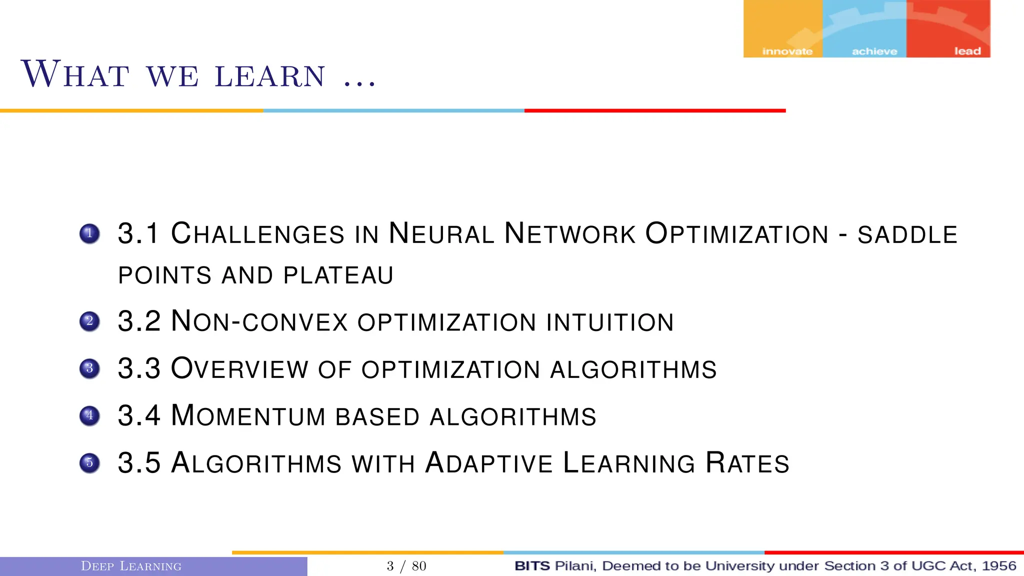
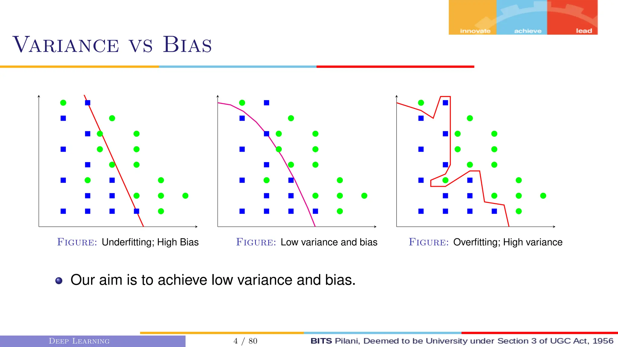
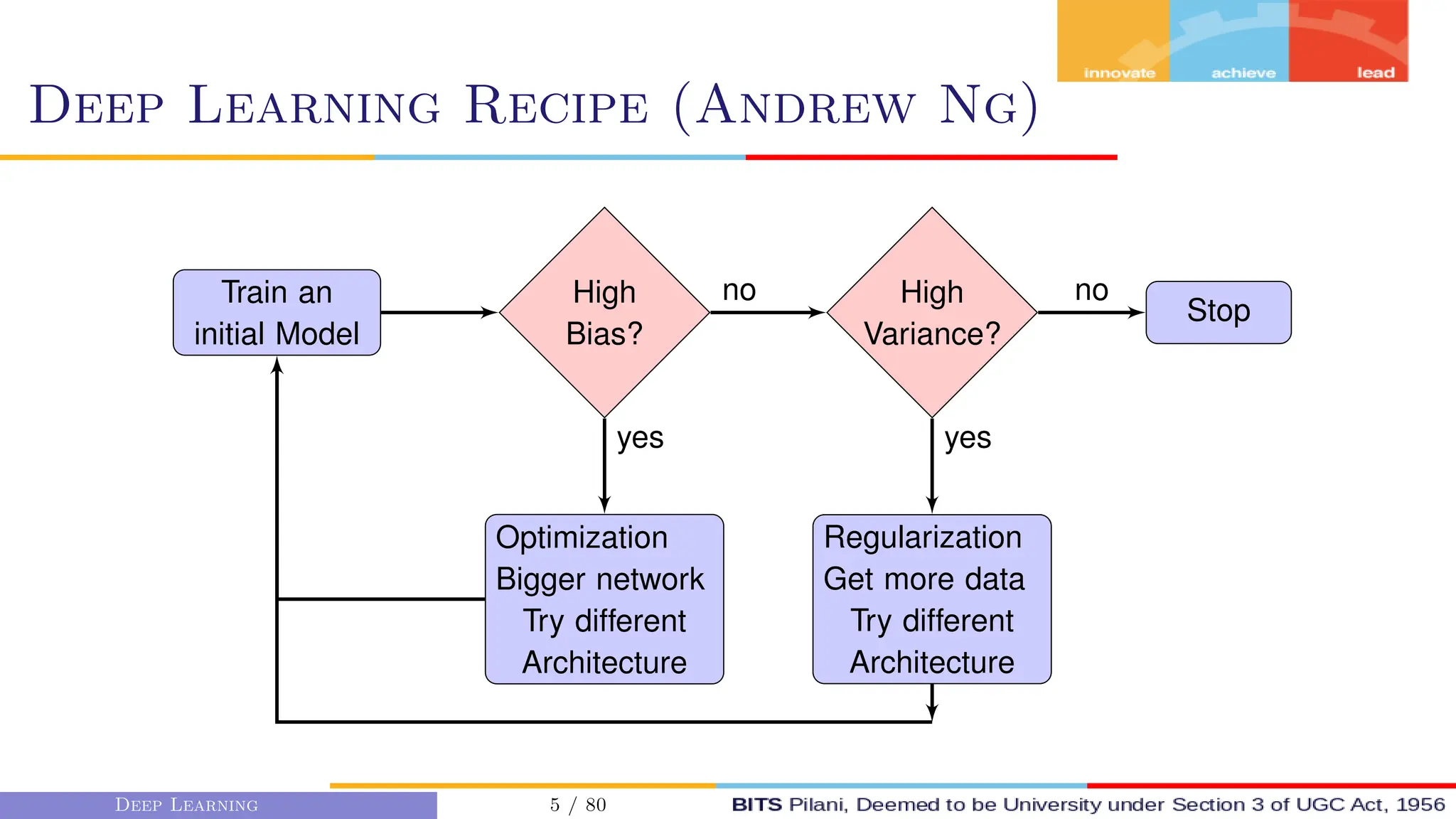
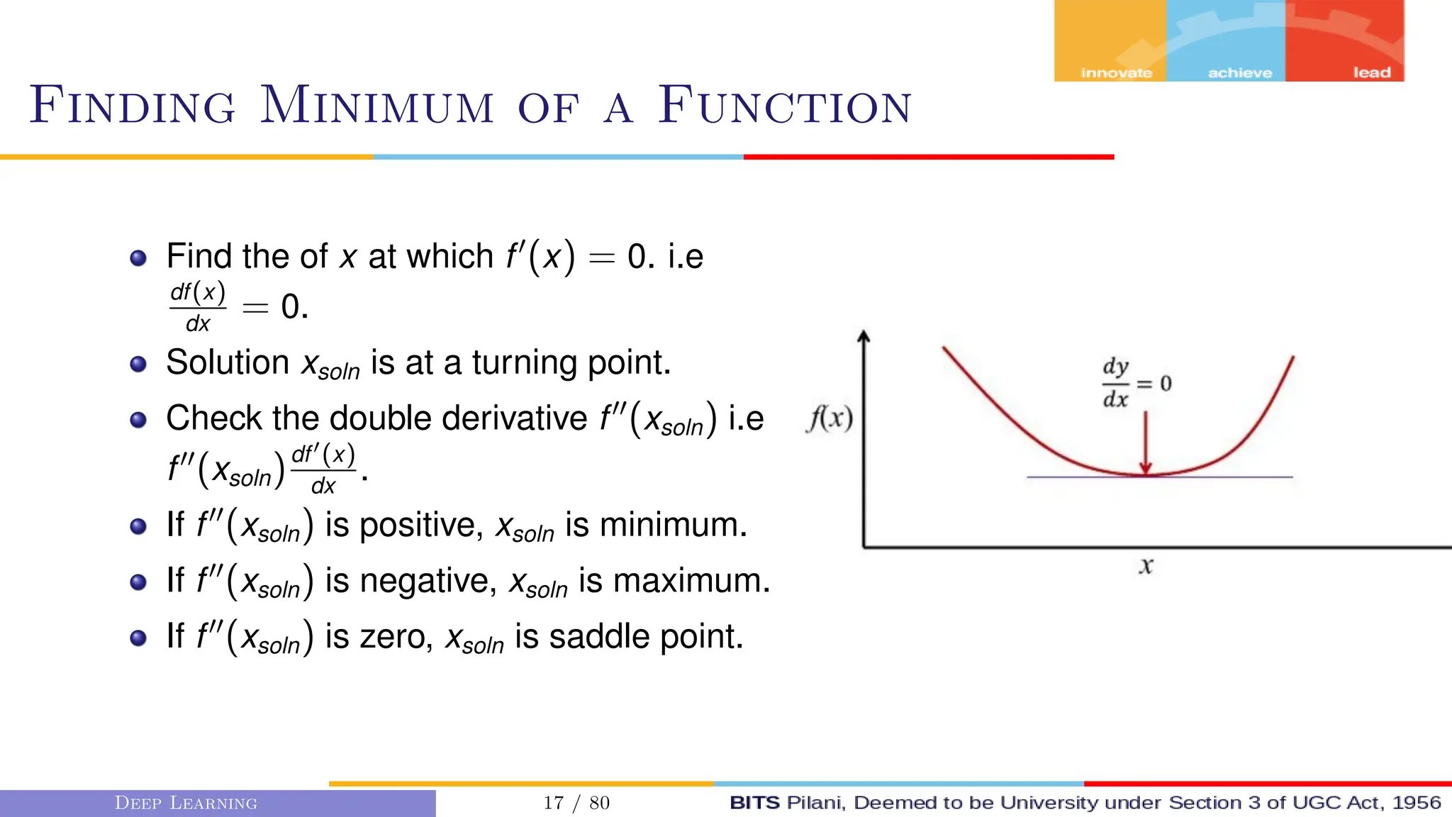
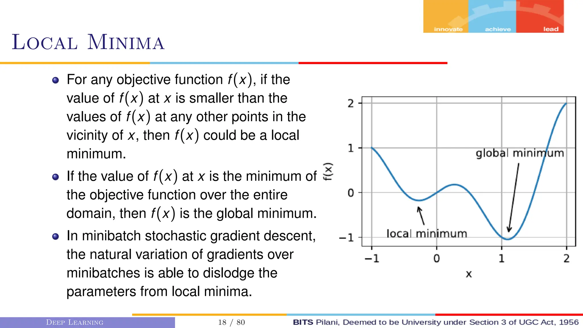
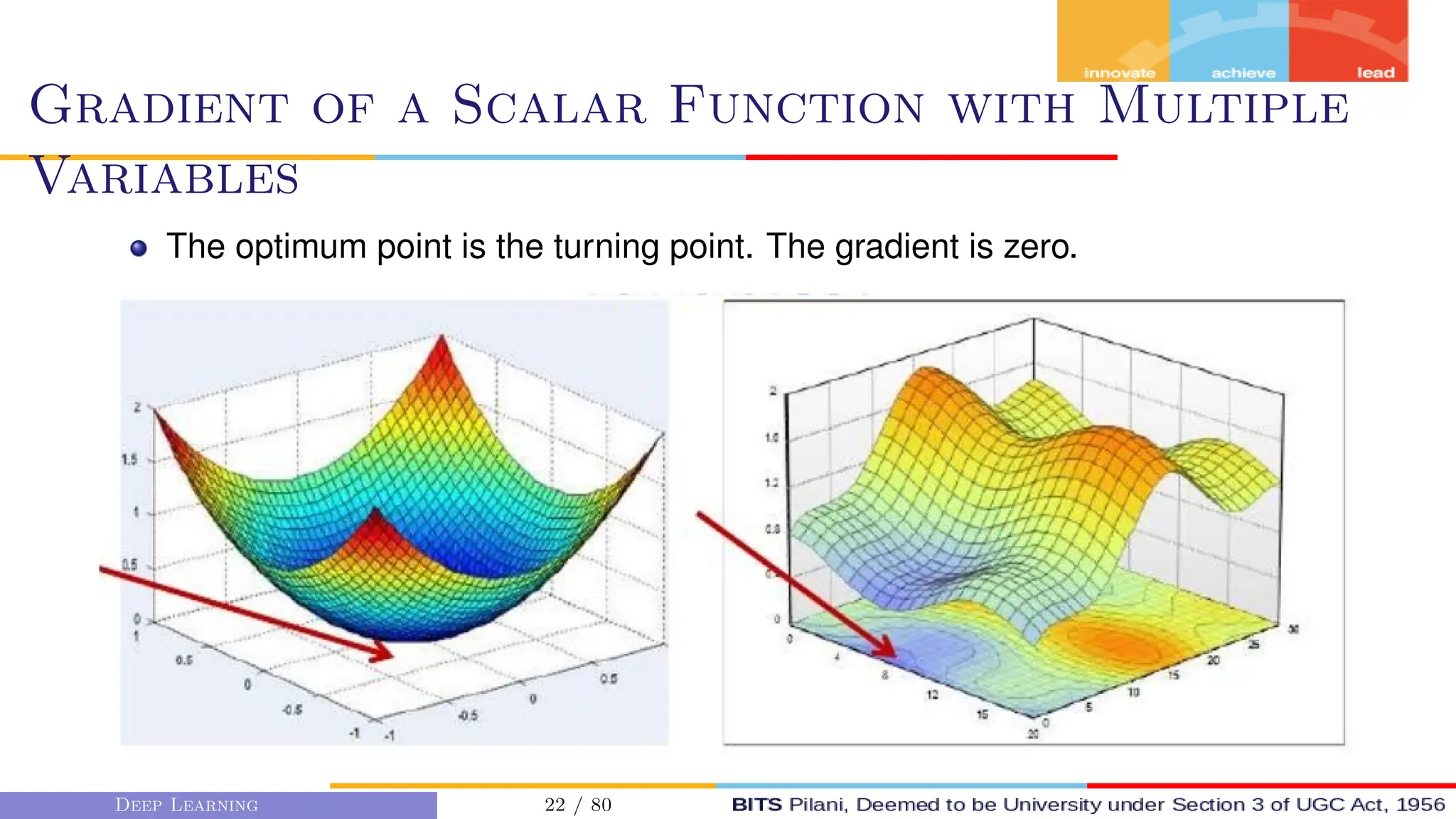
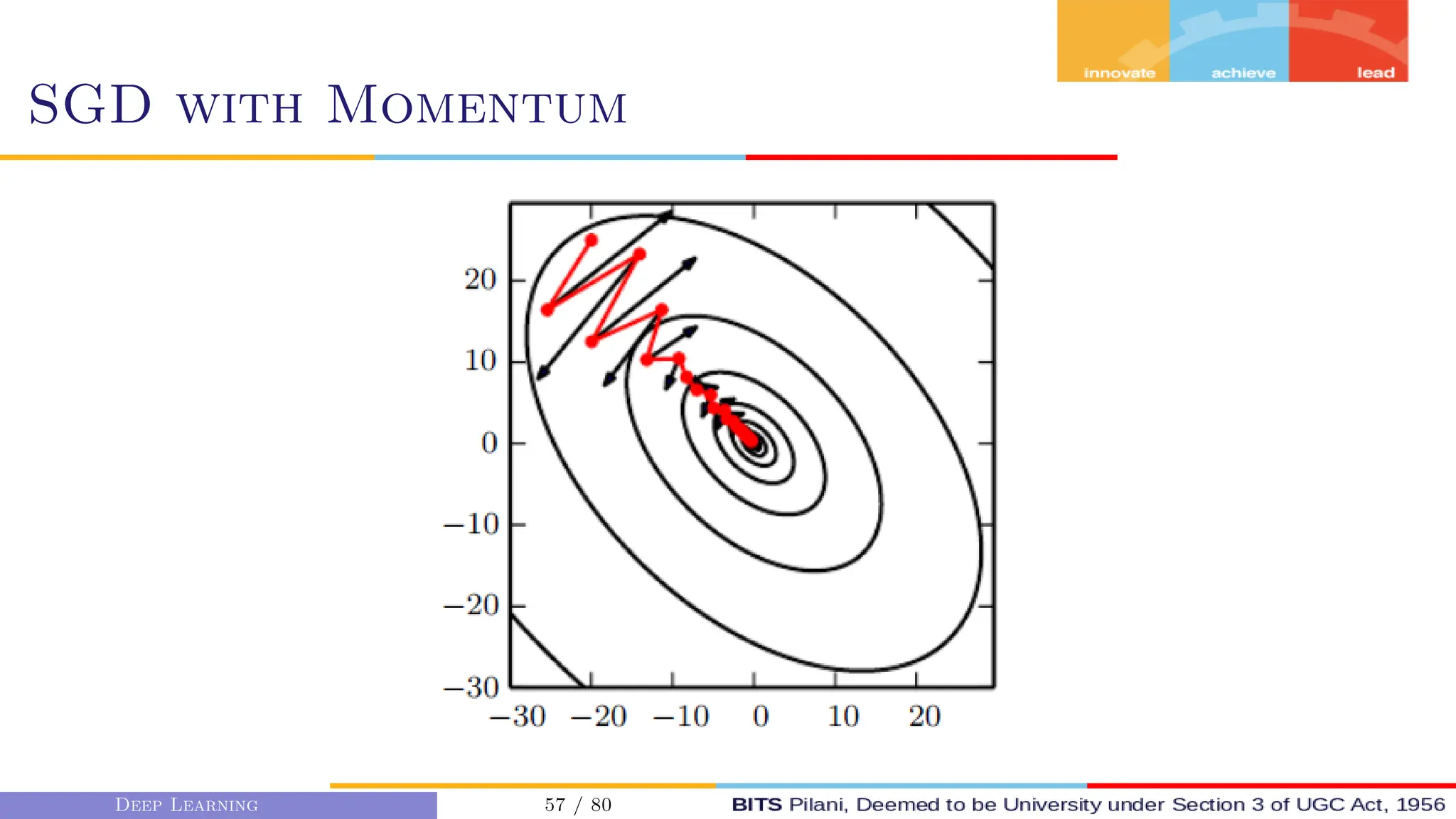
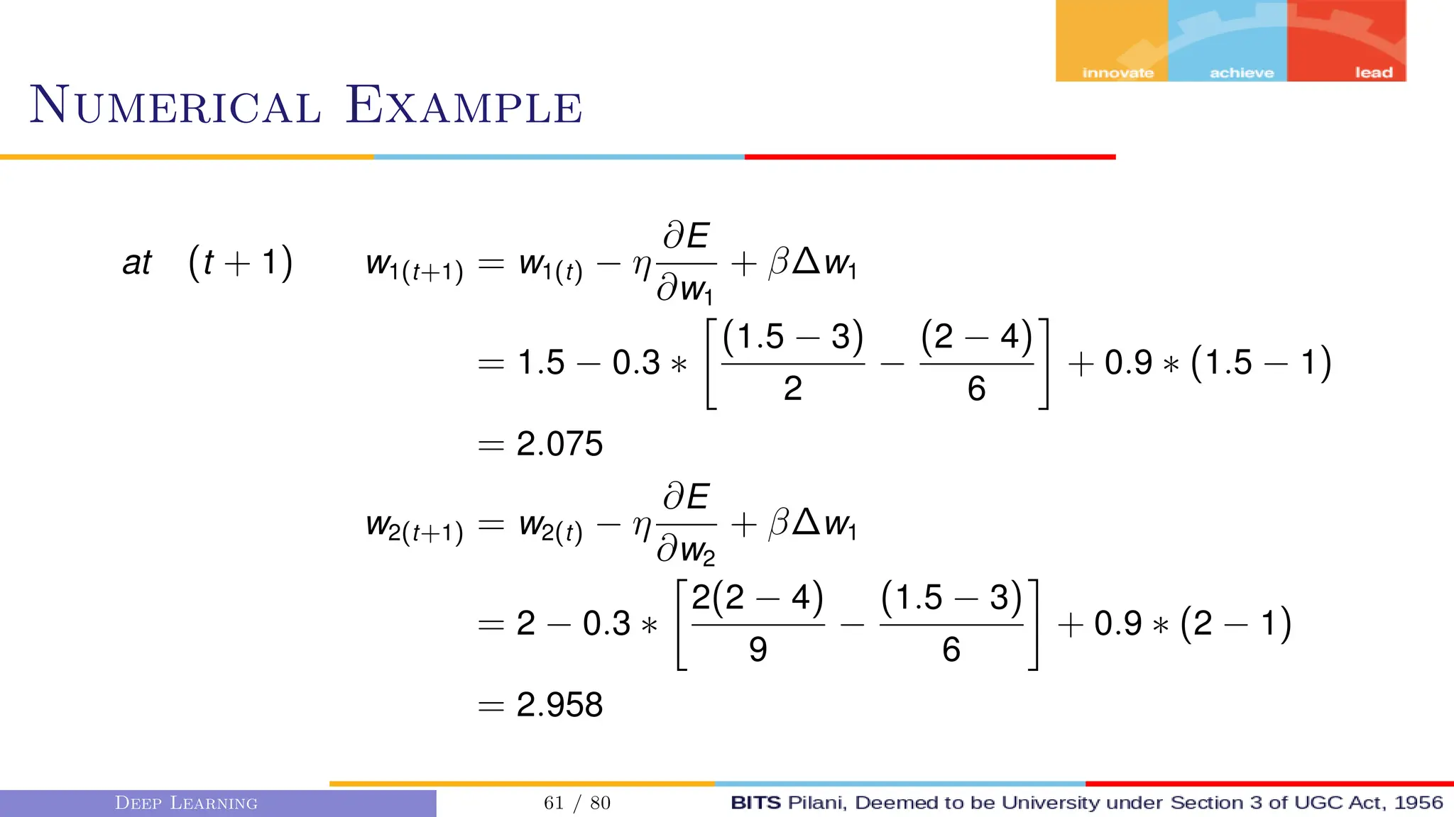
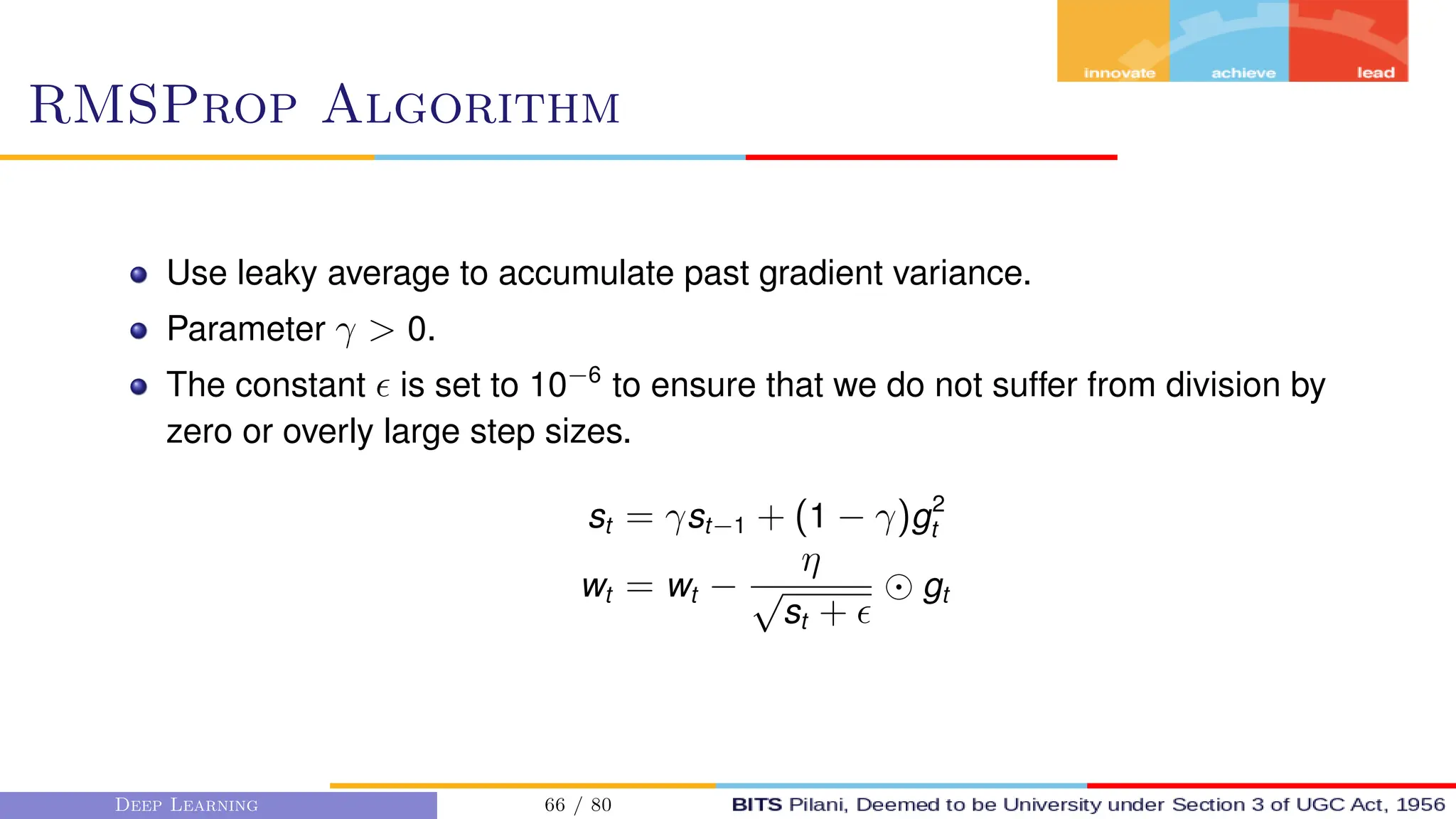
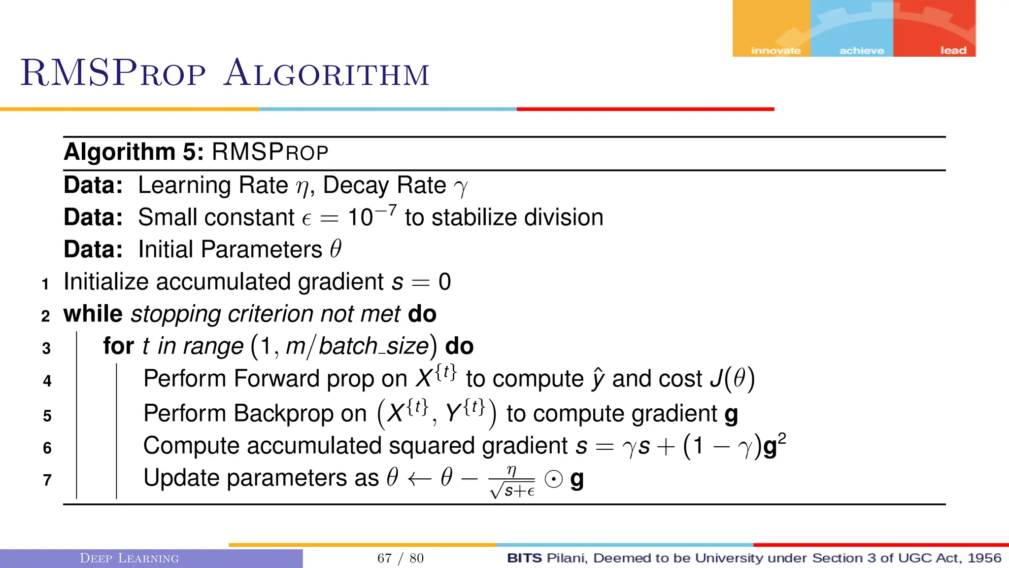
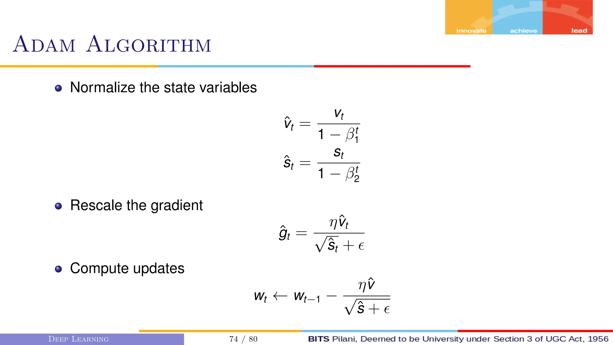
This document provides an overview of optimization techniques for deep learning models. It begins with challenges in neural network optimization such as saddle points and vanishing gradients. It then discusses various optimization algorithms including gradient descent, stochastic gradient descent, momentum, Adagrad, RMSProp, and Adam. The goal of optimization algorithms is to train deep learning models by minimizing the loss function through iterative updates of the model parameters. Learning rate, batch size, and other hyperparameters of the algorithms affect how quickly and accurately they can find the minimum.


![Gradient Descent
First order Gradient Descent algos
consider the first order derivatives
to get the magnitude and direction
of update.
def gd ( eta , f grad ) :
x = 10.0
r e s u l t s = [ x ]
f o r i in range ( 1 0 ) :
x −= eta * f grad ( x )
r e s u l t s . append ( f l o a t ( x ) )
return r e s u l t s
Deep Learning 33 / 80](https://image.slidesharecdn.com/dnnm3optimization-240212192030-48ba0d1f/75/DNN_M3_Optimization-pdf-33-2048.jpg)


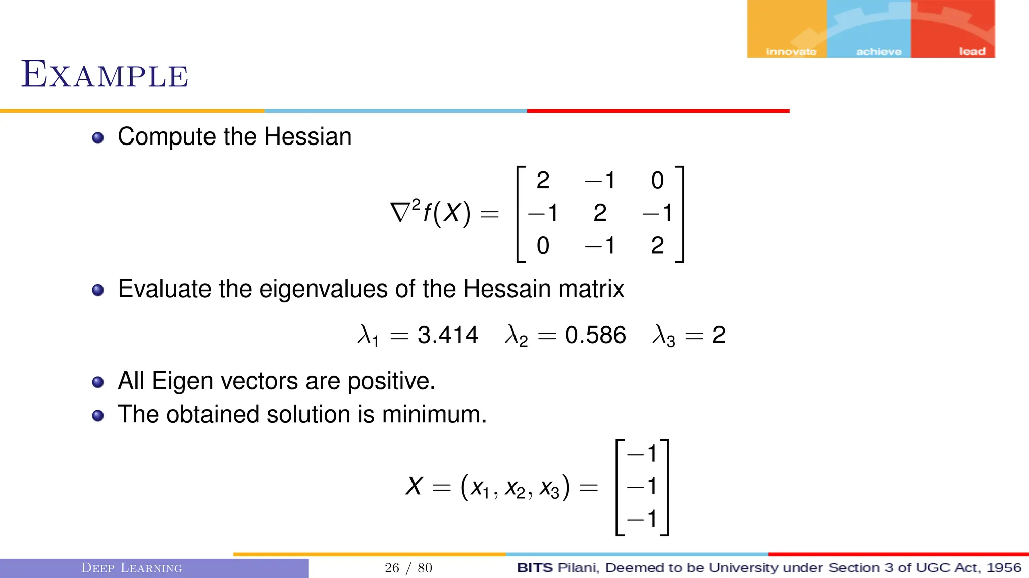
![Example
Error surface is given by E(x, y, z) = 3x2
+2y2
+4z2
+6. Assume gradient descent
is used to find the minimum of this error surface. What is the optimal learning rate
that leads to fastest convergence to the global minimum?
E(x, y, z) = 3x2
+ 2y2
+ 4z2
+ 6
ηxopt = 1/6
ηyopt = 1/4
ηzopt = 1/8
optimal learning rate for convergence = min[ηxopt , ηyopt , ηzopt ] = 1/8
Largest learning rate for convergence = min[2ηxopt , 2ηyopt , 2ηzopt ] = 0.33
Learning rate for divergence 2ηopt = 2 ∗ 1/8 = 0.25
Deep Learning 39 / 80](https://image.slidesharecdn.com/dnnm3optimization-240212192030-48ba0d1f/75/DNN_M3_Optimization-pdf-39-2048.jpg)


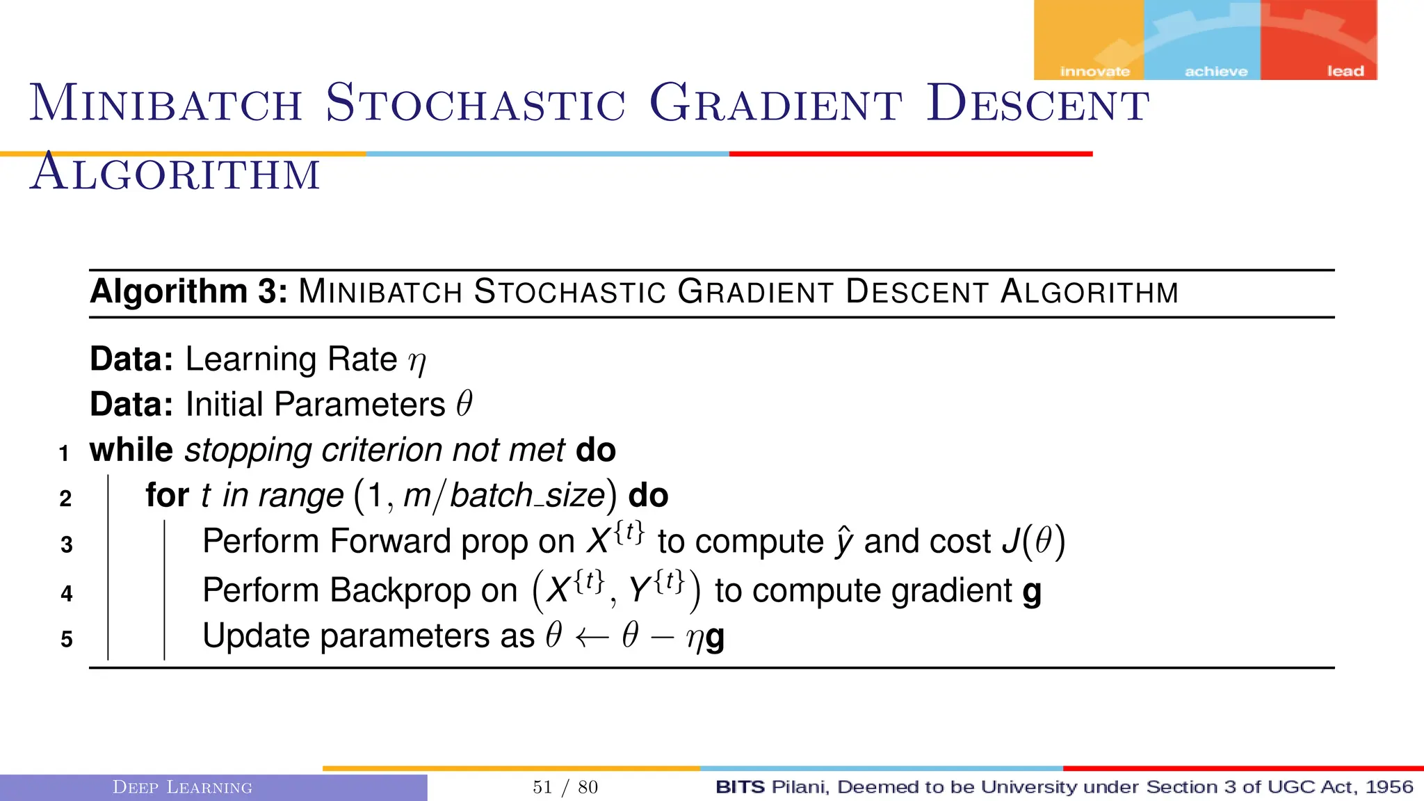
![Minibatch Stochastic Gradient Descent
Suppose we have 4 million examples in the training set.
X = [X(1)
, X(2)
, . . . , X(m)
]
Y = [Y(1)
, Y(2)
, . . . , Y(m)
]
The gradient descent algorithm process the entire dataset of m = 4 million
examples before proceeding to the next step. This is cumbersome and time
consuming.
Hence split the training dataset.
Deep Learning 47 / 80](https://image.slidesharecdn.com/dnnm3optimization-240212192030-48ba0d1f/75/DNN_M3_Optimization-pdf-47-2048.jpg)
![Minibatch Stochastic Gradient Descent
Let the mini-batch size be 1000.
Then we have 4000 mini-batches, each having 1000 examples.
X = [X(1)
, X(2)
, . . . , X(m)
]
= [X(1)
, X(2)
, . . . , X(1000)
, X(1001)
, . . . , X(2000)
, . . . , X(m)
]
= X{1}
, X{2}
, . . . , X{m/b}
Y = [Y(1)
, Y(2)
, . . . , Y(m)
]
= [Y(1)
, Y(2)
, . . . , Y(1000)
, Y(1001)
, . . . , Y(2000)
, . . . , Y(m)
]
= Y{1}
, Y{2}
, . . . , Y{m/b}
The minibatch t is denoted as X{t}
, Y{t}
The Gradient descent algorithm will be repeated for t batches.
Deep Learning 48 / 80](https://image.slidesharecdn.com/dnnm3optimization-240212192030-48ba0d1f/75/DNN_M3_Optimization-pdf-48-2048.jpg)


![Numerical Example
Forward Pass and Calculate Loss
ŷ = σ(wx + b) = σ(−2.0 × 3.5 − 2.0) ≈ 0.0180
L = −[y × log(ŷ) + (1 − y) × log(1 − ŷ)
L = −[0.5 × log(0.0180) + (1 − 0.5) × log(1 − 0.0180)] ≈ 4.0076
Calculate Gradients
∇w L = (ŷ − y) × x = (0.0180 − 0.5) × 3.5 ≈ −0.493
∇bL = ŷ − y = 0.0180 − 0.5 ≈ −0.482
Update First Moments
sW = β1 × sW + (1 − β1) × ∇w L = 0.90 × 0 − 0.10 × (−0.493) ≈ 0.04437
sB = β1 × sB + (1 − β1) × ∇bL = 0.90 × 0 − 0.10 × (−0.482) ≈ 0.04382
Deep Learning 78 / 80](https://image.slidesharecdn.com/dnnm3optimization-240212192030-48ba0d1f/75/DNN_M3_Optimization-pdf-78-2048.jpg)