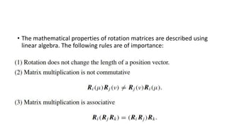
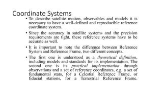
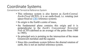
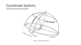
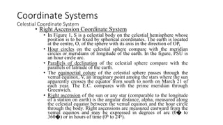
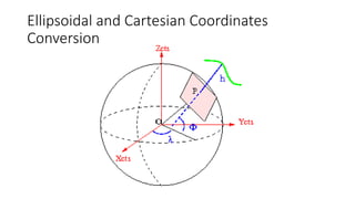
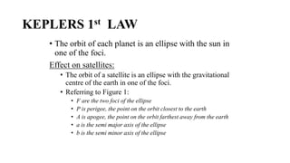
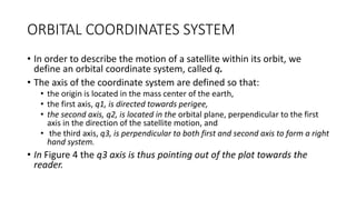
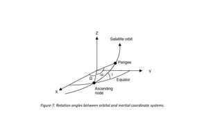
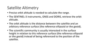
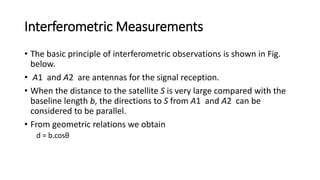
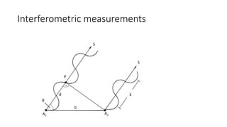
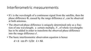
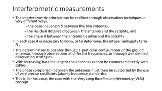
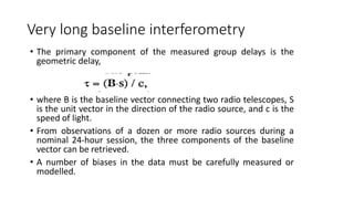
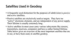
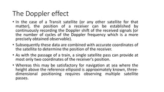
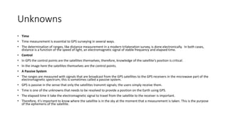
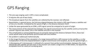
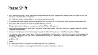
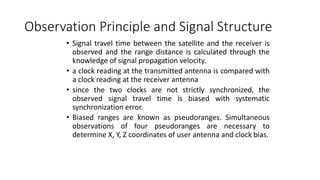
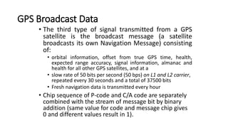
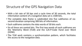
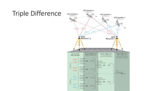
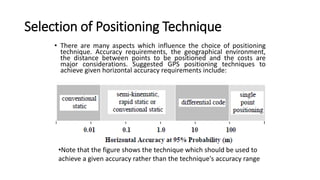
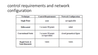
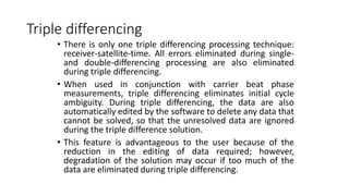
The document discusses satellite geodesy, covering its definition, historical developments, and applications. It outlines the methods and objectives of satellite measurements for geodetic problems, including determining Earth's dimensions and gravity field. The text also details coordinate systems crucial for satellite motions, emphasizing the importance of accurate reference systems and their transformations.


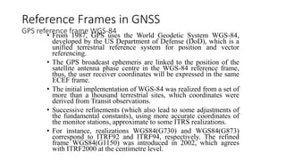
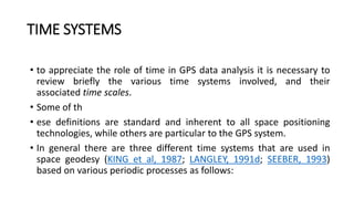
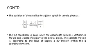
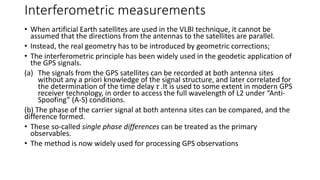
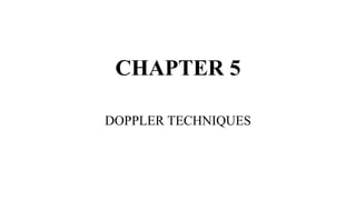
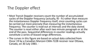
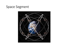
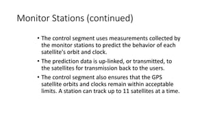
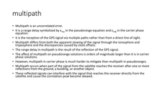
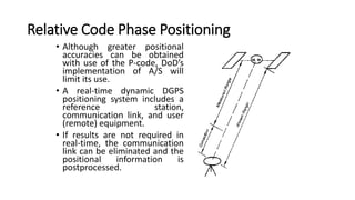
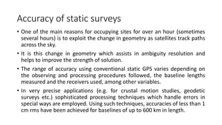
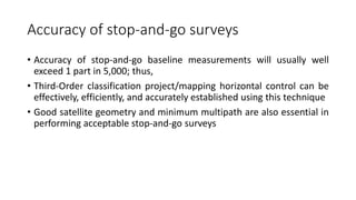
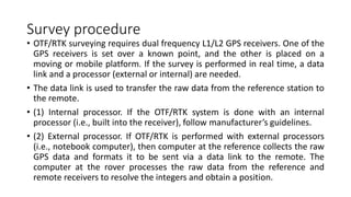
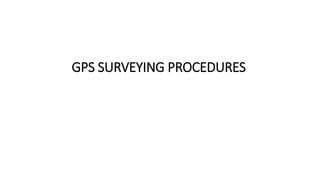
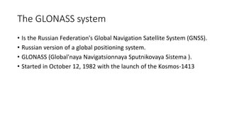
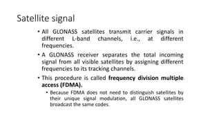
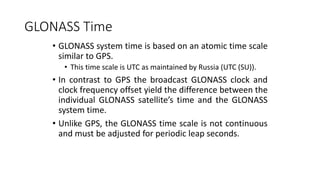
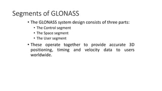
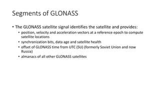
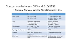
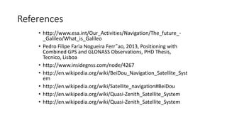
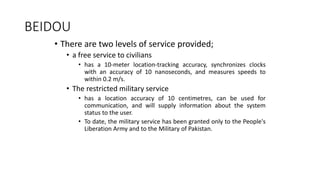
![• The GLONASS broadcast ephemeris are given in the
Parametry Zemli 1990 (Parameters of the Earth 1990) (PZ-
90) reference frame.
• As the WGS-84, this is an ECEF frame with a set of
fundamental parameters associated (see table 2 from
[GLONASS ICD, 2008]).
• The determination of a set of parameters to transform the
PZ-90 coordinates to the ITRF97 was the target of the
International GLONASS Experiment (IGEX-98).
• [Boucher and Altamimi, 2001] presents a review of the
IGEX-98 experiment and, as a conclusion, they suggest
the following transformation from (x,y,z) in PZ-90
to (x',y',z') in WGS-84, with a meter level of accuracy.
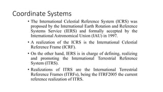
Reference Frames in GNSS
GLONASS reference frame PZ-90](https://image.slidesharecdn.com/satellitegeodesylecturenotesmsu2015-230427055911-8a9b47db/85/Satellite-Geodesy-Lecture-Notes-MSU-2015-pptx-49-320.jpg)
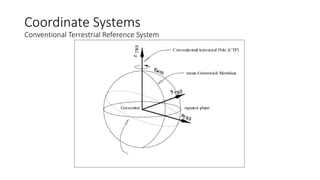
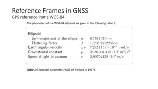
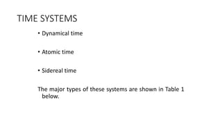
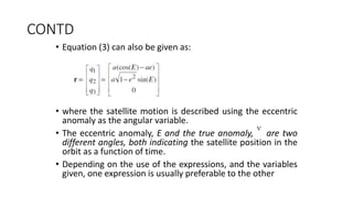
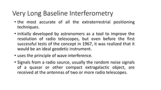
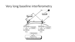
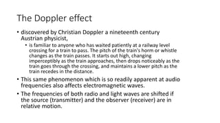
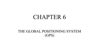
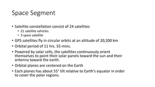
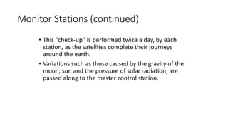
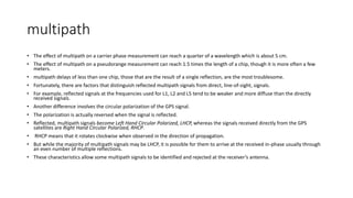
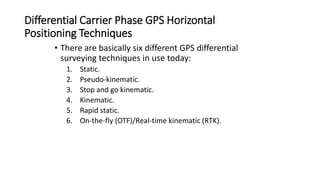
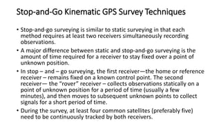
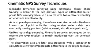
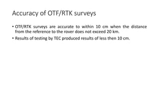
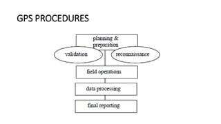
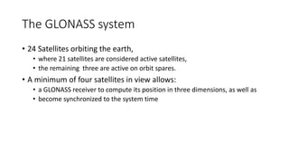
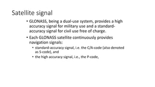
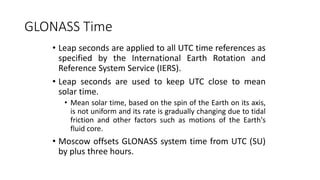
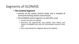
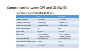
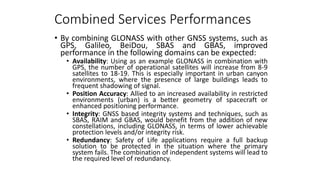
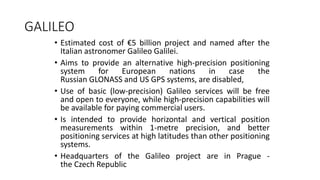
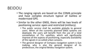
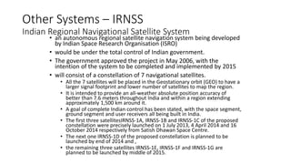
![• According to the GLONASS modernisation plan, the
ephemeris information implementing the PZ-90.02
reference system was updated on all operational
GLONASS satellites from 12:00 to 17:00 UTC,
September 20th., 2007.
• From this time on, the satellites are broadcasting in the
PZ-90.02. This ECEF reference frame is an updated
version of PZ-90, closest to the ITRF2000.
• The transformation from PZ-90.02 to ITRF2000
contains only an origin shift vector, but no rotations
nor scale factor, as it is shown in equation (2)
[Revnivykh, 2007]
Reference Frames in GNSS
GLONASS reference frame PZ-90](https://image.slidesharecdn.com/satellitegeodesylecturenotesmsu2015-230427055911-8a9b47db/85/Satellite-Geodesy-Lecture-Notes-MSU-2015-pptx-51-320.jpg)
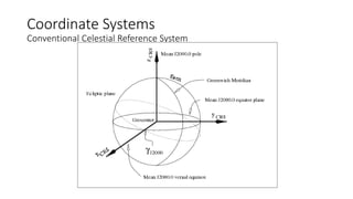
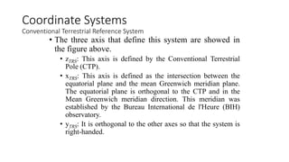
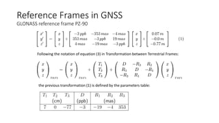
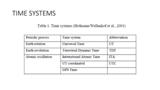
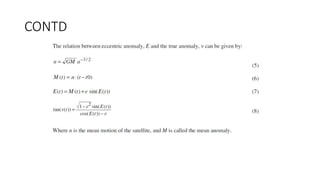
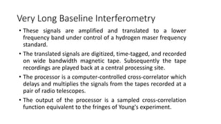
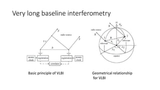
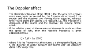
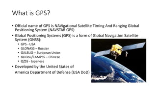
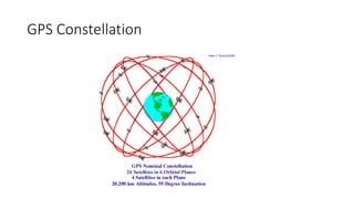
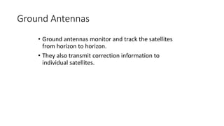
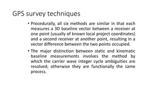
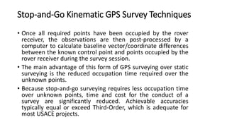
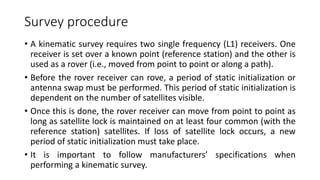
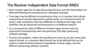
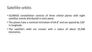
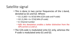
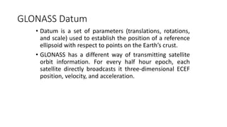
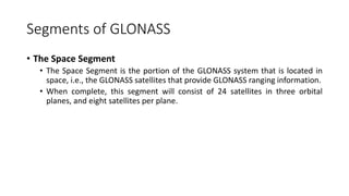
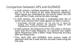
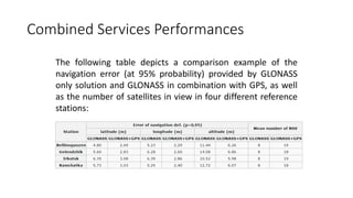
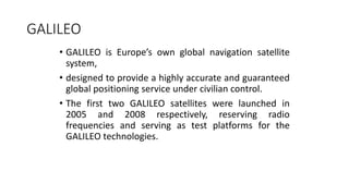
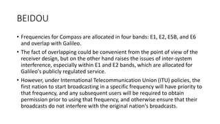
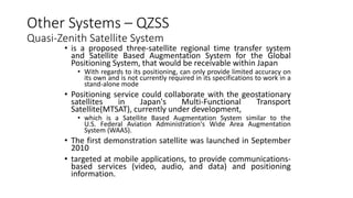
![• The parameters associated to the PZ-90 and PZ-90.02 are
given in the next table 2 ([GLONASS ICD, 1998] and
[GLONASS ICD, 2008]):
Reference Frames in GNSS
GLONASS reference frame PZ-90](https://image.slidesharecdn.com/satellitegeodesylecturenotesmsu2015-230427055911-8a9b47db/85/Satellite-Geodesy-Lecture-Notes-MSU-2015-pptx-53-320.jpg)
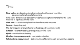
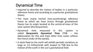
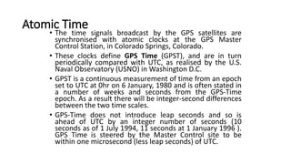
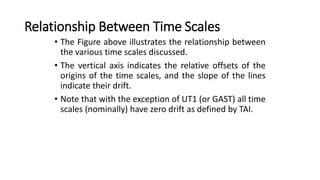
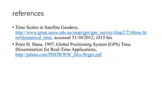
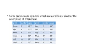
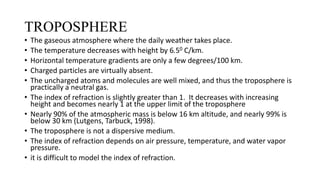
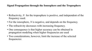
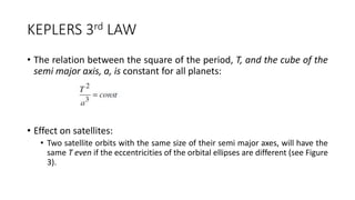
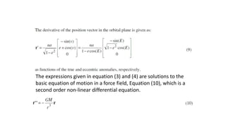
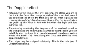
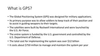
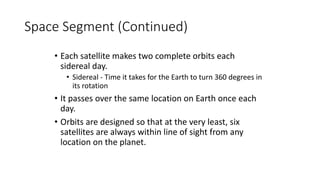
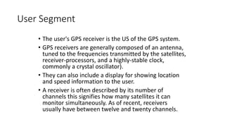
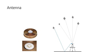
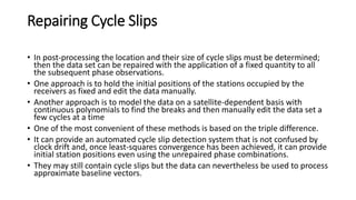
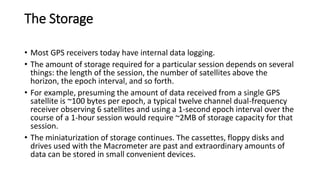
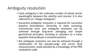
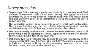
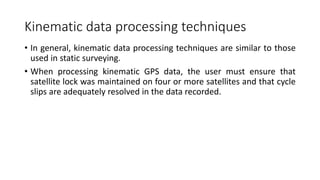
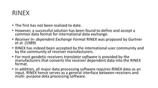
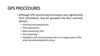
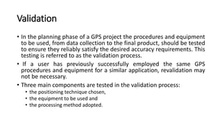
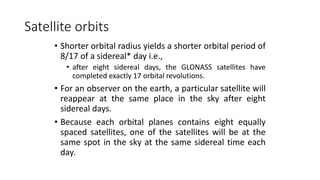
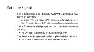
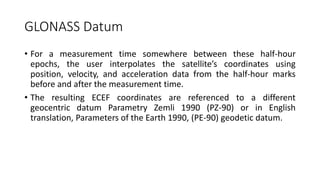
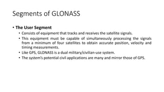
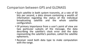
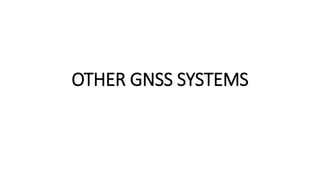
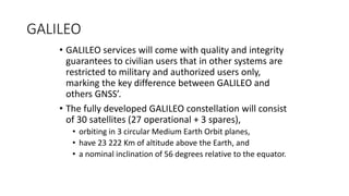
![Cont’d
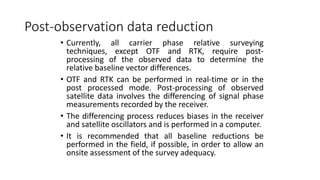
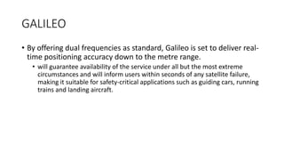
• photo-chemical processes that depend on the insolation of the sun, and govern
the production and de- composition rate of ionized particles, and
• transportation processes that cause a motion of the ionized layers.
• Both processes create different layers of ionized gas at different heights.
• The main layers are known as the D-, E-, F1 -, and F2 -layers. In particular, the F1
-layer, located directly below the F2 -layer, shows large variations that correlate
with the relative sun spot number.
• Geomagnetic influences also play an important role.
• Hence, signal propagation in the ionosphere is severely affected by solar activity,
near the geomagnetic equator, and at high latitudes
• The state of the ionosphere is described by the electron density ne with the unit
[number of electrons/m3 ] or [number of electrons/cm3 ].](https://image.slidesharecdn.com/satellitegeodesylecturenotesmsu2015-230427055911-8a9b47db/85/Satellite-Geodesy-Lecture-Notes-MSU-2015-pptx-91-320.jpg)
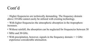
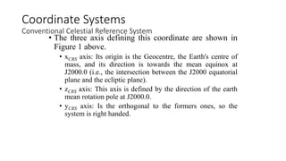
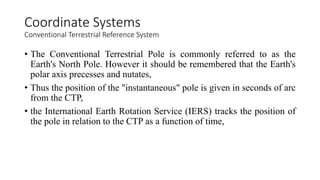
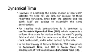
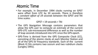
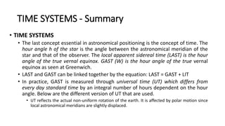
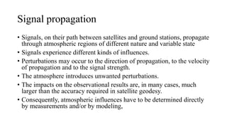
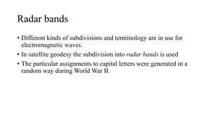
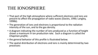
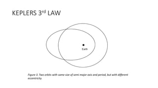
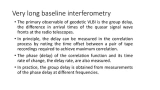
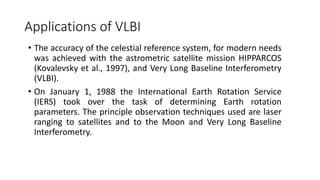
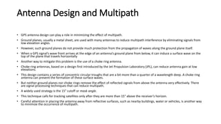
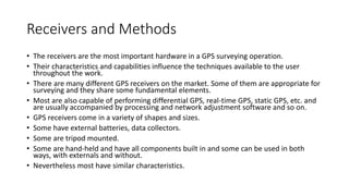
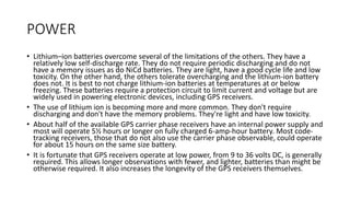
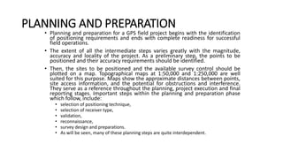
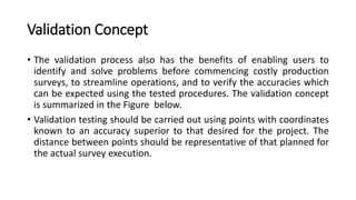
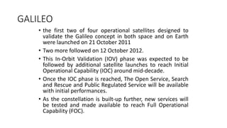
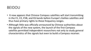
![Implications
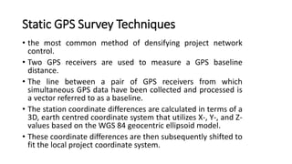
• The selection of frequencies for a particular satellite system is always a
compro- mise.
• This was the case with the TRANSIT system [6] when 150/400 MHz were
selected reflecting the technological progress of the 1960’s.
• And this is true for the GPS system [7] with the selection of 1.2/1.6 GHz.
• Table above gives an impression of how the ionosphere affects the
propagation delay at different frequencies, and it indicates the residual
errors when measurements on two frequencies are available.
• It becomes clear that for the GPS system, operating with two frequencies,
the residual errors are mostly below 1cm.](https://image.slidesharecdn.com/satellitegeodesylecturenotesmsu2015-230427055911-8a9b47db/85/Satellite-Geodesy-Lecture-Notes-MSU-2015-pptx-95-320.jpg)
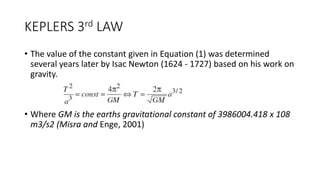

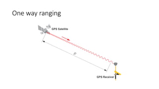
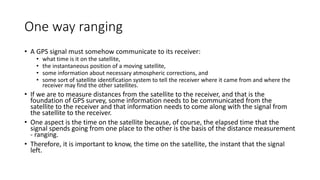
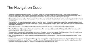
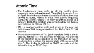
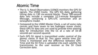
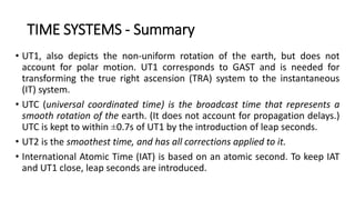
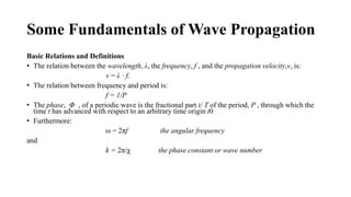
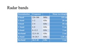
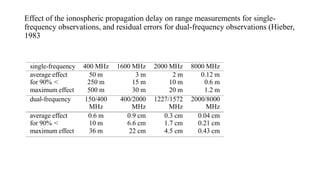
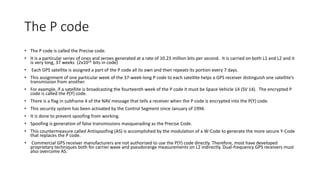
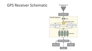
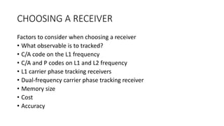
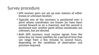
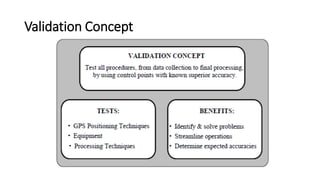
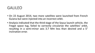
![The Broadcast Ephemeris
• Contain information about the position of the satellite, with respect to time.
• The ephemeris that each satellite broadcasts to the receivers provides information about its position relative
to the earth.
• Most particularly it provides information about the position of the satellite antenna's phase center.
• The ephemeris is given in a right ascension (RA) system of coordinates.
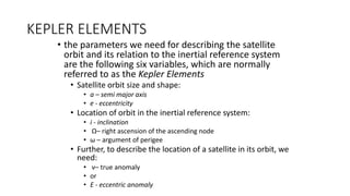
• There are six orbital elements;
• the size of the orbit, that is its semimajor axis, a
• its shape, that is the eccentricity, e.
• the right ascension of its ascending node, Ω,
• the inclination of its plane, i.
• the argument of the perigee, ω,
• The description of the position of the satellite on the orbit, known as the true anomaly,
• provides all the information the user’s computer needs to calculate earth-centered, earth-fixed, World
Geodetic System 1984, GPS Week 1762 (WGS84 [G1762]) coordinates of the satellite at any moment.
• The Control Segment uploads the ephemerides to the Navigation Message for each individual satellite.](https://image.slidesharecdn.com/satellitegeodesylecturenotesmsu2015-230427055911-8a9b47db/85/Satellite-Geodesy-Lecture-Notes-MSU-2015-pptx-223-320.jpg)


![International spheroid[1]](https://cdn.slidesharecdn.com/ss_thumbnails/internationalspheroid1-130817100358-phpapp02-thumbnail.jpg?width=640&height=640&fit=bounds)


![[Deck] What's New in Spark-Iceberg Integration via DSV2.pptx](https://cdn.slidesharecdn.com/ss_thumbnails/deckwhatsnewinspark-icebergintegrationviadsv2-260210005337-25955b12-thumbnail.jpg?width=640&height=640&fit=bounds)


