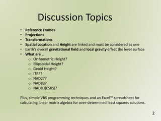
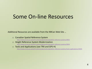
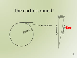
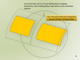
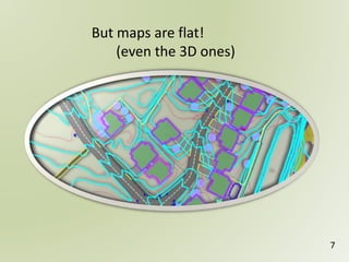
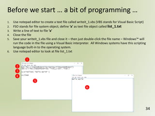
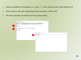
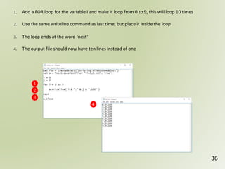
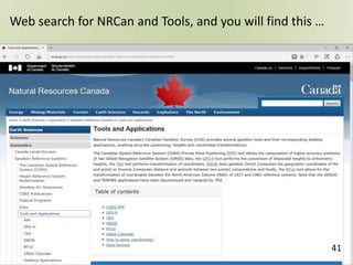
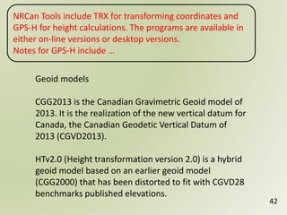
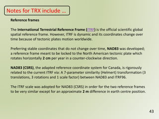
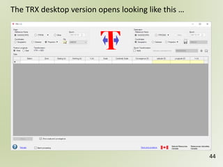
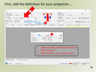
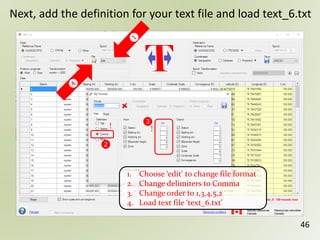
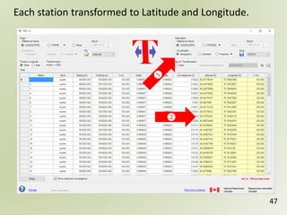
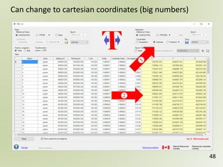
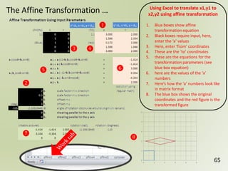
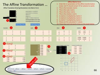
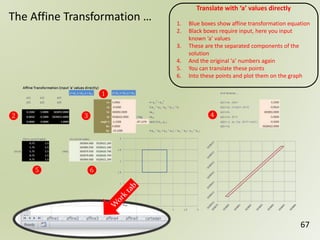
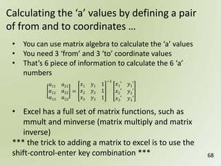
1 2 3 4 51 2 3 4 5
Geospatial
Reference
Systems
1
Introduction
2
• Reference Frames
• Projections
• Transformations
• Spatial Location and Height are linked and must be considered as one
• Earth’s overall gravitational field and local gravity effect the level surface
• What are …
o Orthometric Height?
o Ellipsoidal Height?
o Geoid Height?
o ITRF?
o NAD27?
o NAD83?
o NAD83(CSRS)?
Plus, simple VBS programming techniques and an Excel™ spreadsheet for
calculating linear matrix algebra for over-determined least squares solutions.
Discussion Topics
3
If you’d like a copy of the Excel spreadsheet documented in this presentation, please
request one by sending an email to geospatialreferencesystems@gmail.com
Some On-line Resources
4
Additional Resources are available from the NRCan Web Site …
o Canadian Spatial Reference System
http://www.nrcan.gc.ca/earth-sciences/geomatics/geodetic-reference-systems/9052
o Height Reference System Modernization
http://www.nrcan.gc.ca/earth-sciences/geomatics/geodetic-reference-systems/9054
o Tools and Applications (see TRX and GPS-H)
http://www.nrcan.gc.ca/earth-sciences/geomatics/geodetic-reference-systems/tools-applications/10925
8m per 10 km
The earth is round!
5
6,378,000m
10,000 m
Just to be clear, we’re not just talking about mapping
projections, we’re talking about map datums and coordinate
systems.
The Transverse Mercator Projection
Secant Cylinder Through Globe
6
But maps are flat!
(even the 3D ones)
7
8
There are no straight lines on the curved surface
1 2 3 4 51 2 3 4 5Horizontal vs Vertical
Geospatial
Reference
Systems
9
If the Earth was …
- a perfect sphere
- had uniform gravity
The zenith/nadir line at any
point on the Earth would pass
through the centre of the
Earth.
… and water would not flow in
any direction.
10
11
The Ellipsoid
N
b
a
S
𝑓 =
𝑎 − 𝑏
𝑎
= 𝑓𝑙𝑎𝑡𝑡𝑒𝑛𝑖𝑛𝑔
a = 6,378,137.000 meters (semi-major axis)
b = 6,356,752.3141403 m (semi-minor axis)
1/f = 298.25722210088 (flattening)
f = 0.003352811 (inverse flattening, close to
zero, close to a perfect sphere)
Geodetic Reference System 1980 (GRS80)
a = Semi major axis
b = Semi minor axis
12
Different Inverse Flattening Values …
f = 0 f = 0.2 f = 0.5
Sphere Flat Flatter
(in fact ½ the height )
13
The earth is slightly flatter at the poles …
To make a grid
system ‘fit’ the
earth, an inverse
flattening value of
0.003352811 is
required.
The Ellipsoid
Describes the (slightly)
flattened earth.
Nadir doesn’t pass through
the centre of the earth,
except at the equator and
poles.
14
The ellipsoid pretty accurately describes sea level over the entire earth’s
surface to, on average, ±300 metres.
• To enhance the accuracy of the ellipsoid to represent
sea level, you can add a geoid model
• The equipotential surface of the Earth’s gravity field
which best fits (global)
‘mean sea level’
• Can’t see the surface or measure it directly
• Can be modeled from gravity data
The Geoid …
15
16
For example, the water level at
Vancouver is higher than the water level
at Halifax by 40 to 70 cm.
… oh, and sea level isn’t perfect either!
Geoidal Heights
17
• The geoid is a vertical datum surface
• The Geoid is an equipotential surface
locating the Earth’s local gravitational field
• Represents mean sea level anywhere, not
just over the oceans
• Modelled directly from gravitational
measurements
• A geoidal model must be positioned relative
to an ellipsoid and specific reference frame
(datum)
The Geoid
Because gravity
differs everywhere,
the direction and
angle of local zenith
differs everywhere.
18
The geoid even more accurately describes sea level over the entire
earth’s surface to, on average, ± one metre.
Ontario, Canada is generally
in an area where the geoid is
below the ellipsoid. This
doesn’t mean that Ontario is
below sea level, it just
means that if, for example,
you measured an elevation
with a GPS of 0 metres (or
directly on) the ellipsoid, sea
level would be directly
below that point by the
amount of the geoid.
So, if you measured a GPS
point with an elevation of 20
metres above the ellipsoid,
and the geoid is -20 metres
in that area, the point would
be, yes, 40 metres above sea
level.
19
What if you measured differences in elevation along a straight
line for 10 km and the survey recorded 100 foresight and
backsight measurements … and each time you measured, you
recorded exactly the same backsight and foresight elevation.
Did you measure a perfectly horizontal line?
If it was a north-south line you will have actually measured a
curving line travelling up and down the geoid, but also curving
around the centre of the earth in a shape of an ellipse.
Each of the survey stations will be gravitationally ‘equipotential’
points … water would not flow between them.
Think about this …
20
Surveying in a curvilinear world …
zenith
zenith
zenith
nadir nadir
nadir
8 km
8 m
21
1 2 3 4 51 2 3 4 5Coordinate Systems
Geospatial
Reference
Systems
22
Reference Frames
23
• Most ellipsoids use the same reference system
• For example, Geodetic Reference System 1980 (GRS80)
• Most differences among reference systems are the
definition of the location of the centre of the reference
frame and the orientation of the cartesian coordinate
system
24
Now, let’s talk about
coordinate projections.
These are ‘projections’
of a non-developable
surface (sphere) onto a
‘developable’ surface.
A flat piece of paper is
already ‘developed’. It
can be made to lie flat
on a table. But a curved
piece of paper can also
be laid flat on a table.
It’s developable.
A sphere, on the other
hand cannot be made
to lie flat.
Relative to What?
25
• If you know a latitude and longitude, or an easting or northing, what is
it relative to?
• It is relative to a reference system
• Points in the same reference system are accurate to other points within
the same reference system
• The reference system describes a rotated ellipse and is relative to
something, but what?
• NAD27 is relative to a starting point on Meads Ranch in the middle of
the North American Continent
• NAD83(ORI) is relative to permanent ground points measured between
each other, throughout North America
• Both are closely linked to longitude ‘zero’ through Greenwhich England
and the earth’s equator
• Both are closely linked to the geoid and the centre of mass of the earth
• NAD83(CSRS) and ITRF are almost the same, but are even more closely
linked to the geoid and the centre of mass of the earth
26
NAD27 - only fits a grid to North America
Global
Positioning
System
… using Cartesian coordinates …
27
There are no backsight and foresight measurements
GPS does not measure with respect to gravity
GPS only measures straight base-lines between points and
relative to the GPS ground network and satellite constellation
Initially, inside the GPS equipment, the calculations for
measurements are performed in a Cartesian coordinate system,
X, Y, Z coordinates
The ultimate values for the survey stations are output as
longitude, latitude and elevation above the ellipsoid
Height above sea level can be estimated by using a geoid model
For GPS measurements …
28
HN
h
negative
geoid
height
positive
geoid
height
topography
geoid
ellipsoid
Geoid Model
h = ellipsoidal height (from GPS)
N = geoid height (from geoid model)
H = orthometric height (height above sea level)
H = h – N
h = H + N
(to calculate height above sea level using GPS)
29
Earth-Centered-Earth-Fixed Coordinates
(Cartesian Coordinates)
(X,Y,Z)
(0,0,0)
Center of Mass
X
Y
Z
30
Really Large Numbers!
GPS - Derived Ellipsoid Heights


(X,Y,Z) = P (,,h)
h
31
Latitude and Longitude and a
small number for height
32
The ‘old’ coordinate system …
Such as NAD27 and NAD83(ORI)
non-geocentric coordinate system
published historic ground control
separate vertical control network
The ‘new’ coordinate system …
Such as NAD83(CSRS)
active 3-dimensional geocentric coordinate system
an ellipsoid and geoid
defined centre of mass of the earth
ITRF velocities for epochs
Active control
1 2 3 4 51 2 3 4 5
Geospatial
Reference
Systems
33
TRX, GPS-H and VBS
34
Before we start … a bit of programming …
❶
❷
❸
❹
❺
1. Use notepad editor to create a text file called writeit_1.vbs (VBS stands for Visual Basic Script)
2. FSO stands for file system object; define ‘a’ as text file object called list_1.txt
3. Write a line of text to file ‘a’
4. Close the file
5. Save your writeit_1.vbs file and close it – then just double-click the file name – Windows™ will
run the code in the file using a Visual Basic interpreter. All Windows systems have this scripting
language built-in to the operating system.
6. Use notepad editor to look at file list_1.txt
❻
35
1. Add two variables to the program, an ‘i’ and a ‘j’ – at the moment, they’re both defined as 0
2. Write i and j to a file, add a separating comma, and add a ‘,100’ as well
3. The new output file will contain one line as shown below
❶
❷
❸
36
❶
❷
❸
❹
1. Add a FOR loop for the variable i and make it loop from 0 to 9, this will loop 10 times
2. Use the same writeline command as last time, but place it inside the loop
3. The loop ends at the word ‘next’
4. The output file should now have ten lines instead of one
37
❶
❷
1. Add a loop for the ‘j’ variable inside the loop for the ‘i’ variable, yes, you can do that.
2. Using the same writeline command inside the two loops will now create 100 lines of output.
38
❶
❷
1. Now, we will concentrate on changing the ‘i’ and ‘j’ variable into numbers that we should
recognize as a set of geographic projected coordinates. In this case, multiply by 1000 and add
either 360000 or 5030000 depending on whether it’s an easting or northing number.
2. The output will look like a list of 100 different coordinate values.
39
❶
❷
1. For the next step (using TRX and GPS-H) we also need to add a sequential point number and the
word ‘mymtm’
2. The output file, ‘text_6.txt’ will now look like this … you will need this file in the next step.
40
1. VBS stands for Visual Basic Script and is very powerful. If you’ve ever had to find and replace a
text string within a text file, this script will do it very quickly and totally automated.
2. It is included here as just another example of a simple (but very convenient) VBS program.
This VBS code
41
Web search for NRCan and Tools, and you will find this …
42
Geoid models
CGG2013 is the Canadian Gravimetric Geoid model of
2013. It is the realization of the new vertical datum for
Canada, the Canadian Geodetic Vertical Datum of
2013 (CGVD2013).
HTv2.0 (Height transformation version 2.0) is a hybrid
geoid model based on an earlier geoid model
(CGG2000) that has been distorted to fit with CGVD28
benchmarks published elevations.
NRCan Tools include TRX for transforming coordinates and
GPS-H for height calculations. The programs are available in
either on-line versions or desktop versions.
Notes for GPS-H include …
43
Reference frames
The International Terrestrial Reference Frame (ITRF) is the official scientific global
spatial reference frame. However, ITRF is dynamic and its coordinates change over
time because of tectonic plates motion worldwide.
Preferring stable coordinates that do not change over time, NAD83 was developed;
a reference frame meant to be locked to the North American tectonic plate which
rotates horizontally 2 cm per year in a counter-clockwise direction.
NAD83 (CSRS), the adapted reference coordinate system for Canada, is rigorously
related to the current ITRF via: A 7-parameter similarity (Helmert) transformation (3
translations, 3 rotations and 1 scale factor) between NAD83 and ITRF96.
The ITRF scale was adopted for NAD83 (CSRS) in order for the two reference frames
to be very similar except for an approximate 2 m difference in earth centre position.
Notes for TRX include …
44
The TRX desktop version opens looking like this …
45
First, add the definition for your projection …
❷
❸
1. Open custom projection definition
2. Edit ‘mymtm’
3. Add mymtm, 76.5, 304800 and 3°
46
Next, add the definition for your text file and load text_6.txt
❷
!!
1. Choose ‘edit’ to change file format
2. Change delimiters to Comma
3. Change order to 1,3,4,5,2
4. Load text file ‘text_6.txt’
❸
47
Each station transformed to Latitude and Longitude.
48
Can change to cartesian coordinates (big numbers)
49
Can change MTM (what we started with!)
50
Can change UTM (by defining your UTM zone)
To note, Transverse Mercator coordinates are only
defined by the central meridian, false easting and
northing and zone size / scale factor
51
h = ellipsoidal height (from GPS)
N = geoid height (from geoid model)
H = orthometric height (height above sea level)
You use the GPS-H Program the same way …
52
You can also get the reverse
calculation as well, sea level
values to ellipsoidal height
1 2 3 4 51 2 3 4 5
Geospatial
Reference
Systems
53
Transformations
This section will examine the following
transformations;
54
Lat/Long <<to>> MTM or UTM and return
Lat/Long/Elev <<to>> X,Y,Z Cartesian and return
Lat/Long/Elev <<to>> Local Coordinates and return
2-Dimensional Affine transformation
3-Dimensional Affine transformation
For Transverse Mercator …
55
UTM is a 6 degree zone
MTM is a 3 degree zone
6° gives a scale factor at the central meridian of 0.9996
3° gives a scale factor at the central meridian of 0.9999
You need to specify a central longitude and latitude
You need to specify an easting and northing offset
56
❶
❷
❸
❹
❺
❻
Using Excel to translate
Latitude and Longitude values
to X and Y Transverse Mercator
Projected Coordinates
1. black boxes require input
(this requires decimal degrees)
2. these are the parameters
required for a transverse
mercator projection
3. these are the parameters for
the ellipsoid
4. these are the calculated
coordinates
5. here you can translate the
coordinates backwards
6. and here are the original values
7. once again, the rows at the
bottom are included for
multiple point calculations
Using Excel to transform to Transverse Mercator…
For Cartesian Coordinate Transformation …
57
• Remember, X,Y,Z will typically be large numbers
• Point 0,0,0 is at the centre of the earth
• The X axis direction is oriented towards Greenwich
England but at the equator, off the coast of west Africa
• The Y direction is oriented 90° counter-clockwise and to
the equator (somewhere off of south Asia)
• The Z direction is through the north pole
• Depending on where you are on the surface of the earth,
‘up’ isn’t relative to gravity at all, in fact, only at the north
pole is ‘up’ the same as gravity
• In the following example, instead of using an earth sized
sphere, a 1000 m radius sphere is used with an inverse
flattening of 0, thus making it a perfectly round (small)
sphere
58
❶
❷
❸
❹
❺
❻
❼
Using Excel to translate Latitude, Longitude
and Height values to X, Y, Z cartesian
coordinates
1. black boxes require input, decimal degrees
2. to define an ellipsoid, you only need a semi-
major axis and an inverse flattening value
3. in this example, the ellipsoid is a perfect
sphere with radius of 1000 m
4. these are the calculated coordinates, notice
they’re small – because the sphere is only 1000
metres in radius!
5. here you can translate the coordinates
backwards
6. these values should be what you started with
7. the bottom row can be used to translate
multiple points
Using Excel to Transform to Cartesian Coordinates …
59
Or you could write a VBS program …
For a Local Coordinate Transformation …
60
• you pick a single point (lat/long) as a central reference point
• at this point, you calculate the Cartesian coordinate
• also, you calculate a surface normal, a direction straight ‘up’
from the ellipsoid, this will be the z axis direction
• the x axis direction is oriented directly east from this point
• the y axis direction is oriented directly north from this point
• all other points are then transformed relative to the
reference point
• the local coordinates are typically small numbers
• ‘up’ is intuitive and is (almost) generally ‘up’ relative to
gravity
• the transformation includes a 3-dimensional rotation and a
shift, but no scale factor
LOCAL
COORDINATES …
61
Cartesian coordinates,
much smaller numbers!
62
❶ ❷
❸
❹
❺
❻
Using Excel to translate
Latitude and Longitude values
to Local Coordinates
1. You start with a reference
point
2. these are the parameters
required for the ellipsoid
3. This is the reference point in
Cartesian coordinates
4. this is the point to translate
5. This is the point in Cartesian
coordinates
6. and here are the local
coordinates
7. The local coordinate can be
transformed back using the
rotation matrix, but in its
transposed state
8. once again, the rows at the
bottom are included for
multiple point calculations
Using Excel to transform to local coordinates …
❼
❽
63
The Affine Transformation
• The affine transformation can be a conformal
transformation preserving angles
• A shear or skew factor will introduce a factor that warps
angles
• A 2-dimensional transformation works with a single x,y
coordinate
• There is a factor for scale in x and y
• There is a factor for shift in x and y
• There is a rotation of the entire coordinate system
• There can be a skew factor in x and y
64
The 2-Dimensional Affine Transformation
• You can start with the scale, shift, skew and rotation
parameters and work out the transformation ‘a’ factors
• You can use coordinate math or matrix algebra to
perform the transformation
x’ = a11 x + a12 y + a13
y’ = a21 x + a22 y + a23
• The ‘a’ values define the transformation
• In matrix notation …
𝑥′
𝑦′
1
=
𝑎11 𝑎12 𝑎13
𝑎21 𝑎22 𝑎23
𝑥
𝑦
1
65
The Affine Transformation …
❶
❷
❸ ❹
❺ ❻
Using Excel to translate x1,y1 to
x2,y2 using affine transformation
1. Blue boxes show affine
transformation equation
2. Black boxes require input, here,
enter the ‘a’ values
3. Here, enter ‘from’ coordinates
4. These are the ‘to’ coordinates
5. these are the equations for the
transformation parameters (see
blue box equation)
6. here are the values of the ‘a’
numbers
7. Here’s how the ‘a’ numbers look like
in matrix format
8. The blue box shows the original
coordinates and the red figure is the
transformed figure
❼
❽
66
The Affine Transformation …
❶
❷ ❸ ❹ ❺
❻=(2x3)
Affine Matrix Form
1. Enter the ‘a’ parameters of the affine transformation
(note: red ‘0’ should remain ‘0’ for solution to work)
2. This is the translate matrix
3. This is the scale matrix
4. This is the shear matrix
5. This is the rotation matrix
6. Is matrix 2 multiplied by matrix 3
7. Is matrix 6 multiplied by matrix 4
8. Is matrix 7 multiplied by matrix 5
9. These are the calculated ‘a’ values
10. These blue and red points show on the graph below
❿
❾
❼=(6x4)
❽=(7x5)
67
The Affine Transformation …
❶
❷ ❸ ❹
❺ ❻
Translate with ‘a’ values directly
1. Blue boxes show affine transformation equation
2. Black boxes require input, here you input
known ‘a’ values
3. These are the separated components of the
solution
4. And the original ‘a’ numbers again
5. You can translate these points
6. Into these points and plot them on the graph
68
Calculating the ‘a’ values by defining a pair
of from and to coordinates …
• You can use matrix algebra to calculate the ‘a’ values
• You need 3 ‘from’ and 3 ‘to’ coordinate values
• That’s 6 piece of information to calculate the 6 ‘a’
numbers
• Excel has a full set of matrix functions, such as
mmult and minverse (matrix multiply and matrix
inverse)
*** the trick to adding a matrix to excel is to use the
shift-control-enter key combination ***
𝑎11 𝑎21
𝑎12 𝑎22
𝑎13 𝑎23
=
𝑥1 𝑦1 1
𝑥2 𝑦2 1
𝑥3 𝑦3 1
−1
𝑥1′ 𝑦1′
𝑥2′ 𝑦2′
𝑥3′ 𝑦3′
69
3-points to 3-points affine transformation …
❶ ❷
❸
❹
❺
1. 3 ‘from’ coordinates
2. 3 ‘to’ coordinates
3. These are the ‘a’ number solutions
calculated below, see 4
4. Linear matrix solution of ‘a’
numbers
5. Translate a new point using the
same matrix answer
70
What if you have more than 3 ‘from’ and
‘to’ sets of coordinates …
• If you have more than 3 pairs of coordinates, you have an ‘over-
determined’ solution
• One way to solve an over-determined solution is to use a least-square
matrix algebra solution
x = (ATA)-1ATm
• The excel spreadsheet shows how to construct the matrix elements
• This solution is specifically for two sets of 8 – 2-dimensional points
*** it is not that easy to change the dimension of matrix solutions in
excel once they have been added using the shift-control-enter
method ***
71
The Over-Determined
Affine Transformation …
❶ ❷ ❸
❹
❺ ❻
1. These are the eight sets of ‘from’ coordinates
2. These are the eight sets of ‘to’ coordinates
3. Notice all values are the same in this example except point 3
4. These are the ‘a’ values
5. This is a 9th check ‘from’ point
6. This is the 9th check ‘to’ point
7. These are the constructed matrix elements for the translation
8. These are the residuals of the solution, it shows how good the ‘fit’ is
❼
❽
72
The 3-Dimensional Conformal Transformation …
• The solution presented here is an over-determined solution
from one set of 3 – 3-dimensional points to another
corresponding set of 3 – 3-dimensional points
• This is a non-linear solution
• The transformation is calculated by linearizing the non-linear
solution using a Taylor series expansion
• The solution must be given starting estimates
• The least squares solution does not solve the equations, it
only gives numbers that indicate how close to the solution
the input values are
• The matrix ‘answers’ can be added to the initial estimate to
re-calculate a solution
• The answer is ‘solved’ when the matrix ‘answers’ approach ‘0’
73
The 3-Dimensional Conformal Transformation …
• When a matrix answer finds a solution to a non-linear equation, it
is said that the answer ‘converges’ on a solution
• If the initial estimates are good (close to the real answer)
convergence can happen quickly (ie. in only a few iterations)
• Sometimes a solution does not converge, it will diverge, the
‘answers’ will become bigger and bigger, and no solution is found
• Sometimes a solution will converge, but to an incorrect answer
• Care must be taken to examine and check the results from the
solution to ensure that a correct solution has been reached
• For instance, checking that the scale factor is close to 1 (when that
is what is expected) is an easy check when verifying the solution
74
The 3-Dimensional Conformal Transformation …
• Remember – this spreadsheet solves a non-linear problem
using a linearized answer!
• This means you will have to use an iterative approach to get
the solution
• Enter a initial estimates, get their correction factors
• Add the correction factors to the initial estimates and
recalculate
• Repeat until the correction factors are all very small
• Your initial estimates must be close!!
75
The 3D Affine Transformation …
(the seven parameter
3-dimensional transformation)
❶
❷
❸
❹
Using Excel to calculate a 7 parameter
transformation
1. These are the 3 ‘from’ coordinates
2. These are the 3 ‘to’ coordinates
3. Enter initial estimates here
4. Copy the initial estimates into this area
5. Highlight and copy correction factors
from here
6. Paste correction factors here by ‘copy
value’ technique
7. Copy these numbers over top the current
solution – right click and select ‘add’
remember, you want to add these
corrections to the current solution
8. Repeat until corrections are very small
9. These cells are all off screen, you can
ignore them, everything happens in
boxes 5, 6 and 7
❽
❾
❻paste values then copy
❺ copy from here
❼paste add
76
fin

Geospatial reference-systems

  • 1.
    1 2 34 51 2 3 4 5 Geospatial Reference Systems 1 Introduction
  • 2.
    2 • Reference Frames •Projections • Transformations • Spatial Location and Height are linked and must be considered as one • Earth’s overall gravitational field and local gravity effect the level surface • What are … o Orthometric Height? o Ellipsoidal Height? o Geoid Height? o ITRF? o NAD27? o NAD83? o NAD83(CSRS)? Plus, simple VBS programming techniques and an Excel™ spreadsheet for calculating linear matrix algebra for over-determined least squares solutions. Discussion Topics
  • 3.
    3 If you’d likea copy of the Excel spreadsheet documented in this presentation, please request one by sending an email to geospatialreferencesystems@gmail.com
  • 4.
    Some On-line Resources 4 AdditionalResources are available from the NRCan Web Site … o Canadian Spatial Reference System http://www.nrcan.gc.ca/earth-sciences/geomatics/geodetic-reference-systems/9052 o Height Reference System Modernization http://www.nrcan.gc.ca/earth-sciences/geomatics/geodetic-reference-systems/9054 o Tools and Applications (see TRX and GPS-H) http://www.nrcan.gc.ca/earth-sciences/geomatics/geodetic-reference-systems/tools-applications/10925
  • 5.
    8m per 10km The earth is round! 5 6,378,000m 10,000 m
  • 6.
    Just to beclear, we’re not just talking about mapping projections, we’re talking about map datums and coordinate systems. The Transverse Mercator Projection Secant Cylinder Through Globe 6
  • 7.
    But maps areflat! (even the 3D ones) 7
  • 8.
    8 There are nostraight lines on the curved surface
  • 9.
    1 2 34 51 2 3 4 5Horizontal vs Vertical Geospatial Reference Systems 9
  • 10.
    If the Earthwas … - a perfect sphere - had uniform gravity The zenith/nadir line at any point on the Earth would pass through the centre of the Earth. … and water would not flow in any direction. 10
  • 11.
    11 The Ellipsoid N b a S 𝑓 = 𝑎− 𝑏 𝑎 = 𝑓𝑙𝑎𝑡𝑡𝑒𝑛𝑖𝑛𝑔 a = 6,378,137.000 meters (semi-major axis) b = 6,356,752.3141403 m (semi-minor axis) 1/f = 298.25722210088 (flattening) f = 0.003352811 (inverse flattening, close to zero, close to a perfect sphere) Geodetic Reference System 1980 (GRS80) a = Semi major axis b = Semi minor axis
  • 12.
    12 Different Inverse FlatteningValues … f = 0 f = 0.2 f = 0.5 Sphere Flat Flatter (in fact ½ the height )
  • 13.
    13 The earth isslightly flatter at the poles … To make a grid system ‘fit’ the earth, an inverse flattening value of 0.003352811 is required.
  • 14.
    The Ellipsoid Describes the(slightly) flattened earth. Nadir doesn’t pass through the centre of the earth, except at the equator and poles. 14 The ellipsoid pretty accurately describes sea level over the entire earth’s surface to, on average, ±300 metres.
  • 15.
    • To enhancethe accuracy of the ellipsoid to represent sea level, you can add a geoid model • The equipotential surface of the Earth’s gravity field which best fits (global) ‘mean sea level’ • Can’t see the surface or measure it directly • Can be modeled from gravity data The Geoid … 15
  • 16.
    16 For example, thewater level at Vancouver is higher than the water level at Halifax by 40 to 70 cm. … oh, and sea level isn’t perfect either!
  • 17.
    Geoidal Heights 17 • Thegeoid is a vertical datum surface • The Geoid is an equipotential surface locating the Earth’s local gravitational field • Represents mean sea level anywhere, not just over the oceans • Modelled directly from gravitational measurements • A geoidal model must be positioned relative to an ellipsoid and specific reference frame (datum)
  • 18.
    The Geoid Because gravity differseverywhere, the direction and angle of local zenith differs everywhere. 18 The geoid even more accurately describes sea level over the entire earth’s surface to, on average, ± one metre.
  • 19.
    Ontario, Canada isgenerally in an area where the geoid is below the ellipsoid. This doesn’t mean that Ontario is below sea level, it just means that if, for example, you measured an elevation with a GPS of 0 metres (or directly on) the ellipsoid, sea level would be directly below that point by the amount of the geoid. So, if you measured a GPS point with an elevation of 20 metres above the ellipsoid, and the geoid is -20 metres in that area, the point would be, yes, 40 metres above sea level. 19
  • 20.
    What if youmeasured differences in elevation along a straight line for 10 km and the survey recorded 100 foresight and backsight measurements … and each time you measured, you recorded exactly the same backsight and foresight elevation. Did you measure a perfectly horizontal line? If it was a north-south line you will have actually measured a curving line travelling up and down the geoid, but also curving around the centre of the earth in a shape of an ellipse. Each of the survey stations will be gravitationally ‘equipotential’ points … water would not flow between them. Think about this … 20
  • 21.
    Surveying in acurvilinear world … zenith zenith zenith nadir nadir nadir 8 km 8 m 21
  • 22.
    1 2 34 51 2 3 4 5Coordinate Systems Geospatial Reference Systems 22
  • 23.
    Reference Frames 23 • Mostellipsoids use the same reference system • For example, Geodetic Reference System 1980 (GRS80) • Most differences among reference systems are the definition of the location of the centre of the reference frame and the orientation of the cartesian coordinate system
  • 24.
    24 Now, let’s talkabout coordinate projections. These are ‘projections’ of a non-developable surface (sphere) onto a ‘developable’ surface. A flat piece of paper is already ‘developed’. It can be made to lie flat on a table. But a curved piece of paper can also be laid flat on a table. It’s developable. A sphere, on the other hand cannot be made to lie flat.
  • 25.
    Relative to What? 25 •If you know a latitude and longitude, or an easting or northing, what is it relative to? • It is relative to a reference system • Points in the same reference system are accurate to other points within the same reference system • The reference system describes a rotated ellipse and is relative to something, but what? • NAD27 is relative to a starting point on Meads Ranch in the middle of the North American Continent • NAD83(ORI) is relative to permanent ground points measured between each other, throughout North America • Both are closely linked to longitude ‘zero’ through Greenwhich England and the earth’s equator • Both are closely linked to the geoid and the centre of mass of the earth • NAD83(CSRS) and ITRF are almost the same, but are even more closely linked to the geoid and the centre of mass of the earth
  • 26.
    26 NAD27 - onlyfits a grid to North America
  • 27.
  • 28.
    There are nobacksight and foresight measurements GPS does not measure with respect to gravity GPS only measures straight base-lines between points and relative to the GPS ground network and satellite constellation Initially, inside the GPS equipment, the calculations for measurements are performed in a Cartesian coordinate system, X, Y, Z coordinates The ultimate values for the survey stations are output as longitude, latitude and elevation above the ellipsoid Height above sea level can be estimated by using a geoid model For GPS measurements … 28
  • 29.
    HN h negative geoid height positive geoid height topography geoid ellipsoid Geoid Model h =ellipsoidal height (from GPS) N = geoid height (from geoid model) H = orthometric height (height above sea level) H = h – N h = H + N (to calculate height above sea level using GPS) 29
  • 30.
  • 31.
    GPS - DerivedEllipsoid Heights   (X,Y,Z) = P (,,h) h 31 Latitude and Longitude and a small number for height
  • 32.
    32 The ‘old’ coordinatesystem … Such as NAD27 and NAD83(ORI) non-geocentric coordinate system published historic ground control separate vertical control network The ‘new’ coordinate system … Such as NAD83(CSRS) active 3-dimensional geocentric coordinate system an ellipsoid and geoid defined centre of mass of the earth ITRF velocities for epochs Active control
  • 33.
    1 2 34 51 2 3 4 5 Geospatial Reference Systems 33 TRX, GPS-H and VBS
  • 34.
    34 Before we start… a bit of programming … ❶ ❷ ❸ ❹ ❺ 1. Use notepad editor to create a text file called writeit_1.vbs (VBS stands for Visual Basic Script) 2. FSO stands for file system object; define ‘a’ as text file object called list_1.txt 3. Write a line of text to file ‘a’ 4. Close the file 5. Save your writeit_1.vbs file and close it – then just double-click the file name – Windows™ will run the code in the file using a Visual Basic interpreter. All Windows systems have this scripting language built-in to the operating system. 6. Use notepad editor to look at file list_1.txt ❻
  • 35.
    35 1. Add twovariables to the program, an ‘i’ and a ‘j’ – at the moment, they’re both defined as 0 2. Write i and j to a file, add a separating comma, and add a ‘,100’ as well 3. The new output file will contain one line as shown below ❶ ❷ ❸
  • 36.
    36 ❶ ❷ ❸ ❹ 1. Add aFOR loop for the variable i and make it loop from 0 to 9, this will loop 10 times 2. Use the same writeline command as last time, but place it inside the loop 3. The loop ends at the word ‘next’ 4. The output file should now have ten lines instead of one
  • 37.
    37 ❶ ❷ 1. Add aloop for the ‘j’ variable inside the loop for the ‘i’ variable, yes, you can do that. 2. Using the same writeline command inside the two loops will now create 100 lines of output.
  • 38.
    38 ❶ ❷ 1. Now, wewill concentrate on changing the ‘i’ and ‘j’ variable into numbers that we should recognize as a set of geographic projected coordinates. In this case, multiply by 1000 and add either 360000 or 5030000 depending on whether it’s an easting or northing number. 2. The output will look like a list of 100 different coordinate values.
  • 39.
    39 ❶ ❷ 1. For thenext step (using TRX and GPS-H) we also need to add a sequential point number and the word ‘mymtm’ 2. The output file, ‘text_6.txt’ will now look like this … you will need this file in the next step.
  • 40.
    40 1. VBS standsfor Visual Basic Script and is very powerful. If you’ve ever had to find and replace a text string within a text file, this script will do it very quickly and totally automated. 2. It is included here as just another example of a simple (but very convenient) VBS program. This VBS code
  • 41.
    41 Web search forNRCan and Tools, and you will find this …
  • 42.
    42 Geoid models CGG2013 isthe Canadian Gravimetric Geoid model of 2013. It is the realization of the new vertical datum for Canada, the Canadian Geodetic Vertical Datum of 2013 (CGVD2013). HTv2.0 (Height transformation version 2.0) is a hybrid geoid model based on an earlier geoid model (CGG2000) that has been distorted to fit with CGVD28 benchmarks published elevations. NRCan Tools include TRX for transforming coordinates and GPS-H for height calculations. The programs are available in either on-line versions or desktop versions. Notes for GPS-H include …
  • 43.
    43 Reference frames The InternationalTerrestrial Reference Frame (ITRF) is the official scientific global spatial reference frame. However, ITRF is dynamic and its coordinates change over time because of tectonic plates motion worldwide. Preferring stable coordinates that do not change over time, NAD83 was developed; a reference frame meant to be locked to the North American tectonic plate which rotates horizontally 2 cm per year in a counter-clockwise direction. NAD83 (CSRS), the adapted reference coordinate system for Canada, is rigorously related to the current ITRF via: A 7-parameter similarity (Helmert) transformation (3 translations, 3 rotations and 1 scale factor) between NAD83 and ITRF96. The ITRF scale was adopted for NAD83 (CSRS) in order for the two reference frames to be very similar except for an approximate 2 m difference in earth centre position. Notes for TRX include …
  • 44.
    44 The TRX desktopversion opens looking like this …
  • 45.
    45 First, add thedefinition for your projection … ❷ ❸ 1. Open custom projection definition 2. Edit ‘mymtm’ 3. Add mymtm, 76.5, 304800 and 3°
  • 46.
    46 Next, add thedefinition for your text file and load text_6.txt ❷ !! 1. Choose ‘edit’ to change file format 2. Change delimiters to Comma 3. Change order to 1,3,4,5,2 4. Load text file ‘text_6.txt’ ❸
  • 47.
    47 Each station transformedto Latitude and Longitude.
  • 48.
    48 Can change tocartesian coordinates (big numbers)
  • 49.
    49 Can change MTM(what we started with!)
  • 50.
    50 Can change UTM(by defining your UTM zone) To note, Transverse Mercator coordinates are only defined by the central meridian, false easting and northing and zone size / scale factor
  • 51.
    51 h = ellipsoidalheight (from GPS) N = geoid height (from geoid model) H = orthometric height (height above sea level) You use the GPS-H Program the same way …
  • 52.
    52 You can alsoget the reverse calculation as well, sea level values to ellipsoidal height
  • 53.
    1 2 34 51 2 3 4 5 Geospatial Reference Systems 53 Transformations
  • 54.
    This section willexamine the following transformations; 54 Lat/Long <<to>> MTM or UTM and return Lat/Long/Elev <<to>> X,Y,Z Cartesian and return Lat/Long/Elev <<to>> Local Coordinates and return 2-Dimensional Affine transformation 3-Dimensional Affine transformation
  • 55.
    For Transverse Mercator… 55 UTM is a 6 degree zone MTM is a 3 degree zone 6° gives a scale factor at the central meridian of 0.9996 3° gives a scale factor at the central meridian of 0.9999 You need to specify a central longitude and latitude You need to specify an easting and northing offset
  • 56.
    56 ❶ ❷ ❸ ❹ ❺ ❻ Using Excel totranslate Latitude and Longitude values to X and Y Transverse Mercator Projected Coordinates 1. black boxes require input (this requires decimal degrees) 2. these are the parameters required for a transverse mercator projection 3. these are the parameters for the ellipsoid 4. these are the calculated coordinates 5. here you can translate the coordinates backwards 6. and here are the original values 7. once again, the rows at the bottom are included for multiple point calculations Using Excel to transform to Transverse Mercator…
  • 57.
    For Cartesian CoordinateTransformation … 57 • Remember, X,Y,Z will typically be large numbers • Point 0,0,0 is at the centre of the earth • The X axis direction is oriented towards Greenwich England but at the equator, off the coast of west Africa • The Y direction is oriented 90° counter-clockwise and to the equator (somewhere off of south Asia) • The Z direction is through the north pole • Depending on where you are on the surface of the earth, ‘up’ isn’t relative to gravity at all, in fact, only at the north pole is ‘up’ the same as gravity • In the following example, instead of using an earth sized sphere, a 1000 m radius sphere is used with an inverse flattening of 0, thus making it a perfectly round (small) sphere
  • 58.
    58 ❶ ❷ ❸ ❹ ❺ ❻ ❼ Using Excel totranslate Latitude, Longitude and Height values to X, Y, Z cartesian coordinates 1. black boxes require input, decimal degrees 2. to define an ellipsoid, you only need a semi- major axis and an inverse flattening value 3. in this example, the ellipsoid is a perfect sphere with radius of 1000 m 4. these are the calculated coordinates, notice they’re small – because the sphere is only 1000 metres in radius! 5. here you can translate the coordinates backwards 6. these values should be what you started with 7. the bottom row can be used to translate multiple points Using Excel to Transform to Cartesian Coordinates …
  • 59.
    59 Or you couldwrite a VBS program …
  • 60.
    For a LocalCoordinate Transformation … 60 • you pick a single point (lat/long) as a central reference point • at this point, you calculate the Cartesian coordinate • also, you calculate a surface normal, a direction straight ‘up’ from the ellipsoid, this will be the z axis direction • the x axis direction is oriented directly east from this point • the y axis direction is oriented directly north from this point • all other points are then transformed relative to the reference point • the local coordinates are typically small numbers • ‘up’ is intuitive and is (almost) generally ‘up’ relative to gravity • the transformation includes a 3-dimensional rotation and a shift, but no scale factor
  • 61.
  • 62.
    62 ❶ ❷ ❸ ❹ ❺ ❻ Using Excelto translate Latitude and Longitude values to Local Coordinates 1. You start with a reference point 2. these are the parameters required for the ellipsoid 3. This is the reference point in Cartesian coordinates 4. this is the point to translate 5. This is the point in Cartesian coordinates 6. and here are the local coordinates 7. The local coordinate can be transformed back using the rotation matrix, but in its transposed state 8. once again, the rows at the bottom are included for multiple point calculations Using Excel to transform to local coordinates … ❼ ❽
  • 63.
    63 The Affine Transformation •The affine transformation can be a conformal transformation preserving angles • A shear or skew factor will introduce a factor that warps angles • A 2-dimensional transformation works with a single x,y coordinate • There is a factor for scale in x and y • There is a factor for shift in x and y • There is a rotation of the entire coordinate system • There can be a skew factor in x and y
  • 64.
    64 The 2-Dimensional AffineTransformation • You can start with the scale, shift, skew and rotation parameters and work out the transformation ‘a’ factors • You can use coordinate math or matrix algebra to perform the transformation x’ = a11 x + a12 y + a13 y’ = a21 x + a22 y + a23 • The ‘a’ values define the transformation • In matrix notation … 𝑥′ 𝑦′ 1 = 𝑎11 𝑎12 𝑎13 𝑎21 𝑎22 𝑎23 𝑥 𝑦 1
  • 65.
    65 The Affine Transformation… ❶ ❷ ❸ ❹ ❺ ❻ Using Excel to translate x1,y1 to x2,y2 using affine transformation 1. Blue boxes show affine transformation equation 2. Black boxes require input, here, enter the ‘a’ values 3. Here, enter ‘from’ coordinates 4. These are the ‘to’ coordinates 5. these are the equations for the transformation parameters (see blue box equation) 6. here are the values of the ‘a’ numbers 7. Here’s how the ‘a’ numbers look like in matrix format 8. The blue box shows the original coordinates and the red figure is the transformed figure ❼ ❽
  • 66.
    66 The Affine Transformation… ❶ ❷ ❸ ❹ ❺ ❻=(2x3) Affine Matrix Form 1. Enter the ‘a’ parameters of the affine transformation (note: red ‘0’ should remain ‘0’ for solution to work) 2. This is the translate matrix 3. This is the scale matrix 4. This is the shear matrix 5. This is the rotation matrix 6. Is matrix 2 multiplied by matrix 3 7. Is matrix 6 multiplied by matrix 4 8. Is matrix 7 multiplied by matrix 5 9. These are the calculated ‘a’ values 10. These blue and red points show on the graph below ❿ ❾ ❼=(6x4) ❽=(7x5)
  • 67.
    67 The Affine Transformation… ❶ ❷ ❸ ❹ ❺ ❻ Translate with ‘a’ values directly 1. Blue boxes show affine transformation equation 2. Black boxes require input, here you input known ‘a’ values 3. These are the separated components of the solution 4. And the original ‘a’ numbers again 5. You can translate these points 6. Into these points and plot them on the graph
  • 68.
    68 Calculating the ‘a’values by defining a pair of from and to coordinates … • You can use matrix algebra to calculate the ‘a’ values • You need 3 ‘from’ and 3 ‘to’ coordinate values • That’s 6 piece of information to calculate the 6 ‘a’ numbers • Excel has a full set of matrix functions, such as mmult and minverse (matrix multiply and matrix inverse) *** the trick to adding a matrix to excel is to use the shift-control-enter key combination *** 𝑎11 𝑎21 𝑎12 𝑎22 𝑎13 𝑎23 = 𝑥1 𝑦1 1 𝑥2 𝑦2 1 𝑥3 𝑦3 1 −1 𝑥1′ 𝑦1′ 𝑥2′ 𝑦2′ 𝑥3′ 𝑦3′
  • 69.
    69 3-points to 3-pointsaffine transformation … ❶ ❷ ❸ ❹ ❺ 1. 3 ‘from’ coordinates 2. 3 ‘to’ coordinates 3. These are the ‘a’ number solutions calculated below, see 4 4. Linear matrix solution of ‘a’ numbers 5. Translate a new point using the same matrix answer
  • 70.
    70 What if youhave more than 3 ‘from’ and ‘to’ sets of coordinates … • If you have more than 3 pairs of coordinates, you have an ‘over- determined’ solution • One way to solve an over-determined solution is to use a least-square matrix algebra solution x = (ATA)-1ATm • The excel spreadsheet shows how to construct the matrix elements • This solution is specifically for two sets of 8 – 2-dimensional points *** it is not that easy to change the dimension of matrix solutions in excel once they have been added using the shift-control-enter method ***
  • 71.
    71 The Over-Determined Affine Transformation… ❶ ❷ ❸ ❹ ❺ ❻ 1. These are the eight sets of ‘from’ coordinates 2. These are the eight sets of ‘to’ coordinates 3. Notice all values are the same in this example except point 3 4. These are the ‘a’ values 5. This is a 9th check ‘from’ point 6. This is the 9th check ‘to’ point 7. These are the constructed matrix elements for the translation 8. These are the residuals of the solution, it shows how good the ‘fit’ is ❼ ❽
  • 72.
    72 The 3-Dimensional ConformalTransformation … • The solution presented here is an over-determined solution from one set of 3 – 3-dimensional points to another corresponding set of 3 – 3-dimensional points • This is a non-linear solution • The transformation is calculated by linearizing the non-linear solution using a Taylor series expansion • The solution must be given starting estimates • The least squares solution does not solve the equations, it only gives numbers that indicate how close to the solution the input values are • The matrix ‘answers’ can be added to the initial estimate to re-calculate a solution • The answer is ‘solved’ when the matrix ‘answers’ approach ‘0’
  • 73.
    73 The 3-Dimensional ConformalTransformation … • When a matrix answer finds a solution to a non-linear equation, it is said that the answer ‘converges’ on a solution • If the initial estimates are good (close to the real answer) convergence can happen quickly (ie. in only a few iterations) • Sometimes a solution does not converge, it will diverge, the ‘answers’ will become bigger and bigger, and no solution is found • Sometimes a solution will converge, but to an incorrect answer • Care must be taken to examine and check the results from the solution to ensure that a correct solution has been reached • For instance, checking that the scale factor is close to 1 (when that is what is expected) is an easy check when verifying the solution
  • 74.
    74 The 3-Dimensional ConformalTransformation … • Remember – this spreadsheet solves a non-linear problem using a linearized answer! • This means you will have to use an iterative approach to get the solution • Enter a initial estimates, get their correction factors • Add the correction factors to the initial estimates and recalculate • Repeat until the correction factors are all very small • Your initial estimates must be close!!
  • 75.
    75 The 3D AffineTransformation … (the seven parameter 3-dimensional transformation) ❶ ❷ ❸ ❹ Using Excel to calculate a 7 parameter transformation 1. These are the 3 ‘from’ coordinates 2. These are the 3 ‘to’ coordinates 3. Enter initial estimates here 4. Copy the initial estimates into this area 5. Highlight and copy correction factors from here 6. Paste correction factors here by ‘copy value’ technique 7. Copy these numbers over top the current solution – right click and select ‘add’ remember, you want to add these corrections to the current solution 8. Repeat until corrections are very small 9. These cells are all off screen, you can ignore them, everything happens in boxes 5, 6 and 7 ❽ ❾ ❻paste values then copy ❺ copy from here ❼paste add
  • 76.