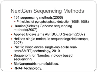
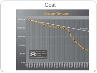
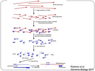
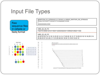
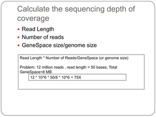
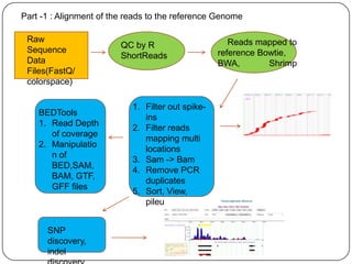
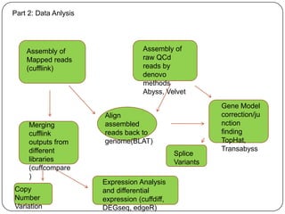
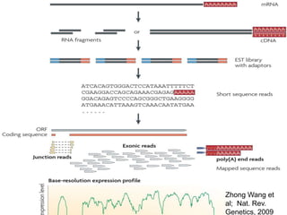
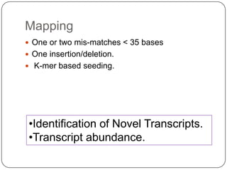
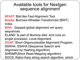
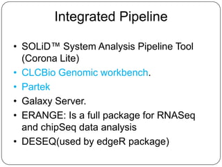
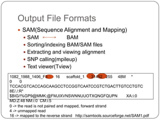
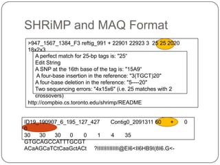
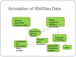
Transcript discovery and
 gene model correction
 using next generation
    sequencing data

    Sucheta Tripathy, 6th July
             2012
NextGen Sequencing Methods
 454 sequencing methods(2006)
     Principles of pyrophosphate detection(1985, 1988)
 Illumina(Solexa) Genome sequencing
    methods(2007)
   Applied Biosystems ABI SOLiD System(2007)
   Helicos single molecule sequencing(Helioscope,
    2007)
   Pacific Biosciences single-molecule real-
    time(SMRT) technology, 2010
   Sequenom for Nanotechnology based
    sequencing.
   BioNanomatrix nanofluidiscs.
   RNAP technology.
Cost
Roberts et al.
Genome Biology 2011
RNASeq
 Catalogue all species of transcripts.
   mRNA
   Non-coding RNA
   Small RNA
 Splicing patterns or other post-transcriptional
  modifications.
 Quantify the expression levels.
Topics covered
 Sequence formats
   Calculate the sequencing depth of coverage
 Data Analysis Workflow
   Mapping programs
     Output data files
       SAM
       SHRIMP
       MAQ
   Clustering and assembly programs
   Finding new genes and correction of existing genes
   Annotation of RNAseq data
Input File Types
                 @SNPSTER4_90_307R0AAXX:2:41:528:604 run=080625_SNPSTER4_090_307R0AAXX
                 GCGCCTATCCACTTTGCGGTCTTCCAAAGNCTCCGG
Raw              +
                 IIIIIIIIIIIIIIIIIIIIIIIIII,II!IIIIII
sequence files
in csfasta or    >853_22_43_F3
                 T32310120021231211023112232332233113303231202211332
fastq format
                 >853_22_43_F3
                 20 24 23 22 14 13 18 12 23 22 14 14 17 26 26 18 12 17 16 26 23 16 15 16 25 5 14
                 25 26 23 8 10 9 20 2 11 2 9 25 26 8 6 19 24 15 18 6 10 20 12
Calculate the sequencing depth of
coverage
 Read Length
 Number of reads
 GeneSpace size/genome size

Read Length * Number of Reads/GeneSpace (or genome size)

Problem: 12 million reads , read length = 50 bases, Total
GeneSpace=8 MB
      12 * 10^6 * 50/8 * 10^6 = 75X
Part -1 : Alignment of the reads to the reference Genome

 Raw                                                  Reads mapped to
                         QC by R
 Sequence                                          reference Bowtie,
                         ShortReads
 Data                                              BWA,        Shrimp
 Files(FastQ/
 colorspace)

                            1. Filter out spike-
    BEDTools
                               ins
    1. Read Depth
                            2. Filter reads
       of coverage
                               mapping multi
    2. Manipulatio
                               locations
       n of
                            3. Sam -> Bam
       BED,SAM,
                            4. Remove PCR
       BAM, GTF,
                               duplicates
       GFF files
                            5. Sort, View,
                               pileup, merge


      SNP
      discovery,
      indel
Part 2: Data Anlysis


    Assembly of                     Assembly of
    Mapped reads                    raw QCd
    (cufflink)                      reads by
                                    denovo
                                    methods
                                    Abyss, Velvet

                                                          Gene Model
                       Align                              correction/ju
     Merging           assembled                          nction
     cufflink          reads back to                      finding
     outputs from      genome(BLAT)                       TopHat,
     different                                            Transabyss
                                               Splice
     libraries                                 Variants
     (cuffcompare
     )
                       Expression Analysis
Copy                   and differential
Number                 expression (cuffdiff,
Variation              DEGseq, edgeR)
Zhong Wang et
al; Nat. Rev.
Genetics, 2009
Mapping
 One or two mis-matches < 35 bases
 One insertion/deletion.
 K-mer based seeding.


 •Identification of Novel Transcripts.
 •Transcript abundance.
Available tools for Nextgen
         sequence alignment
BFAST: Blat like Fast Alignment Tool.
Bowtie: Burrows-Wheeler-Transformed (BWT)
index.
BWA: Gapped global alignment wrt query
sequences.
ELAND: Is part of Illumina distr. And runs on
single processor, Local Alignment.
SOAP: Short Oligonucleotide Alignment Program.
SSAHA: SSAHA (Sequence Search and
Alignment by Hashing Algorithm)
SHRiMP(Short Read Mapping algorithm)
SOCS: Rabin-Karp string search algorithm, which
Integrated Pipeline

• SOLiD™ System Analysis Pipeline Tool
  (Corona Lite)
• CLCBio Genomic workbench.
• Partek
• Galaxy Server.
• ERANGE: Is a full package for RNASeq
  and chipSeq data analysis
• DESEQ(used by edgeR package)
Output File Formats
     SAM(Sequence Alignment and Mapping)
        SAM              BAM
        Sorting/indexing BAM/SAM files
        Extracting and viewing alignment
        SNP calling(mpileup)
        Text viewer(Tview)

1082_1988_1406_F3          16    scaffold_1   31452 255 48M *
0     0
TCCACGTCACCAGCAAGCCTCCGGTCAATCCGTCTGACTTGTCCTGTC
8E/./:R*
$BIG/!%GP9@MMK;@FMJIXVNSWNNUUOTXQNGFQUPN                        XA:i:0
MD:Z:48 NM:i:0 CM:i:5
0 -> the read is not paired and mapped, forward strand
4 -> unmapped read
16 -> mapped to the reverse strand http://samtools.sourceforge.net/SAM1.pdf
SHRiMP and MAQ Format
 >947_1567_1384_F3 reftig_991 + 22901 22923 3 25 25 2020
 18x2x3
    A perfect match for 25-bp tags is: "25“
    Edit String
    A SNP at the 16th base of the tag is: "15A9“
     A four-base insertion in the reference: "3(TGCT)20"
    A four-base deletion in the reference: "5----20"
    Two sequencing errors: "4x15x6" (i.e. 25 matches with 2
    crossovers)
 http://compbio.cs.toronto.edu/shrimp/README


ID19_190907_6_195_127_427     Contig0_2091311 60     +        0
0
30   30   30   0    0   1     4     35
GTGCAGCCATTTGCGT
ACaAGCaTCtCaaGctACt ?IIIIIIIIIIIIII@EI6<II6HB9I(8I6.G<-
Assembly program
 Abyss
   Supports multiple K values
   Fast
   Merging different K valued assembly possible
   Trans-abyss pipeline runs on this


 MIRA(Mimicking Intelligent Read Assembly)
   Hybrid Denovo assembler
   Genome Mapper
 Velvet
Splice Junction prediction
 TopHat
 Cufflink
 MapSplice
 Trans-Abyss
Trapnell et. al 2009
An overview of the MapSplice pipeline.


© The Author(s) 2010. Published by Oxford University Press.

                                                              Wang K et al. Nucl. Acids Res. 2010;38:e178-e178
Denoeud et al,
2008
Cufflink
 Transcript Assembly
 Expression levels with a reference GTF
 Expression levels without GTF.
 Merging experimental replicates(cuffcompare)
 Differential Expression Analysis(cuffdiff)
Annotation of RNASeq Data

   De novo                               Reads
   Assembled                             mapped to
   Reads (contigs)                       reference
                                         assembled

                     Map Back to
                     genome
                     (BLAT)
                                                 Expressio
                            Train for            n Profiling
    Junction/no             gene
    vel                     prediction
    transcripts/                         Differential
    Splice                               Expression            CNV
    variants                             analysis
Genome Viewer
 Desktop/standalone application
     Tbrowse
     Bamview
     Savant
     IGV
     IGB
 Web based browsers
   Gbrowse
   UCSC Genome Browse
   VBI Transcriptomics browser
Other Applications
 SNP detection
 Splice Variant Discovery
 Identification of miRNA targets
 TF binding sites
 Genome Methylation pattern
 RNA editing
 Metagenomic projects
 Gene Expression Analysis
Difference with other expression
sequencing
 EST: Low throughput, expansive, NOT
  quantitative.
 SAGE, CAGE, MPSS: Highthroughput, digital
  gene expression levels
   Expansive
   Sanger sequencing methods
   A portion of transcript is analyzed
   Isoforms are indistinguishable
Advantages:
 Zero or very less background noise.
 Sensitive to isoform discovery.
 Both low and highly expressed genes can be
  quantified.
 Highly reproducible.
Transcripts discovered/Corrected
 10,000 new Transcription start site discovered in
    Rhesus macaque(Liu et al., NAR 2010)
   602 transcriptionally active regions and numerous
    introns in Candida albicans(Bruno et al., 2010,
    Genome Research)
   96% of the genes were corrected in Laccaria
    bicolor(Larsen et al., PLoS One 2010).
   16,923 regions in mouse (Martazavi et al., 2008).
   3,724 novel isoforms (Trapanell 2010).
Bioinformatics Challenges
 Store , retrieve and analyze large amounts of
  data
 Matching of reads to multiple locations
 Short reads with higher copy number and long
  reads representing less expressed genes.
References:
 Wilhelm J. Ansorge, Next-generation DNA sequencing techniques, New
    Biotechnology, Volume 25, Issue 4, April 2009, Pages 195-203
   Zhong Wang, Mark Gerstein, and Michael Snyder. RNA-Seq: a
    revolutionary tool for transcriptomics. Nat Rev Genet. 2009 January;
    10(1): 57–63.
   Peter E. Larsen et al., Using Deep RNA Sequencing for the Structural
    Annotation of the Laccaria Bicolor Mycorrhizal TranscriptomePLoS One.
    2010; 5(7): e9780
   Wang et al. MapSplice: Accurate mapping of RNA-seq reads for splice
    junction discovery, NAR, 2010
   Denoeud et al., Annotating genomes with massive-scale RNA
    sequencing, Genome Biology, 2008
   Trapnell C, Williams BA, Pertea G, Mortazavi AM, Kwan G, van Baren
    MJ, Salzberg SL, Wold B, Pachter L. Transcript assembly and
    quantification by RNA-Seq reveals unannotated transcripts and isoform
    switching during cell differentiation Nature Biotechnology
    doi:10.1038/nbt.1621
   Trapnell C, Pachter L, Salzberg SL. TopHat: discovering splice junctions
    with RNA-Seq. Bioinformatics doi:10.1093/bioinformatics/btp120
   Mortazavi et al. Nature Methods, May 2008

Rnaseq forgenefinding

  • 1.
    Transcript discovery and gene model correction using next generation sequencing data Sucheta Tripathy, 6th July 2012
  • 2.
    NextGen Sequencing Methods 454 sequencing methods(2006)  Principles of pyrophosphate detection(1985, 1988)  Illumina(Solexa) Genome sequencing methods(2007)  Applied Biosystems ABI SOLiD System(2007)  Helicos single molecule sequencing(Helioscope, 2007)  Pacific Biosciences single-molecule real- time(SMRT) technology, 2010  Sequenom for Nanotechnology based sequencing.  BioNanomatrix nanofluidiscs.  RNAP technology.
  • 3.
  • 4.
  • 5.
    RNASeq  Catalogue allspecies of transcripts.  mRNA  Non-coding RNA  Small RNA  Splicing patterns or other post-transcriptional modifications.  Quantify the expression levels.
  • 6.
    Topics covered  Sequenceformats  Calculate the sequencing depth of coverage  Data Analysis Workflow  Mapping programs  Output data files  SAM  SHRIMP  MAQ  Clustering and assembly programs  Finding new genes and correction of existing genes  Annotation of RNAseq data
  • 7.
    Input File Types @SNPSTER4_90_307R0AAXX:2:41:528:604 run=080625_SNPSTER4_090_307R0AAXX GCGCCTATCCACTTTGCGGTCTTCCAAAGNCTCCGG Raw + IIIIIIIIIIIIIIIIIIIIIIIIII,II!IIIIII sequence files in csfasta or >853_22_43_F3 T32310120021231211023112232332233113303231202211332 fastq format >853_22_43_F3 20 24 23 22 14 13 18 12 23 22 14 14 17 26 26 18 12 17 16 26 23 16 15 16 25 5 14 25 26 23 8 10 9 20 2 11 2 9 25 26 8 6 19 24 15 18 6 10 20 12
  • 8.
    Calculate the sequencingdepth of coverage  Read Length  Number of reads  GeneSpace size/genome size Read Length * Number of Reads/GeneSpace (or genome size) Problem: 12 million reads , read length = 50 bases, Total GeneSpace=8 MB 12 * 10^6 * 50/8 * 10^6 = 75X
  • 9.
    Part -1 :Alignment of the reads to the reference Genome Raw Reads mapped to QC by R Sequence reference Bowtie, ShortReads Data BWA, Shrimp Files(FastQ/ colorspace) 1. Filter out spike- BEDTools ins 1. Read Depth 2. Filter reads of coverage mapping multi 2. Manipulatio locations n of 3. Sam -> Bam BED,SAM, 4. Remove PCR BAM, GTF, duplicates GFF files 5. Sort, View, pileup, merge SNP discovery, indel
  • 10.
    Part 2: DataAnlysis Assembly of Assembly of Mapped reads raw QCd (cufflink) reads by denovo methods Abyss, Velvet Gene Model Align correction/ju Merging assembled nction cufflink reads back to finding outputs from genome(BLAT) TopHat, different Transabyss Splice libraries Variants (cuffcompare ) Expression Analysis Copy and differential Number expression (cuffdiff, Variation DEGseq, edgeR)
  • 11.
    Zhong Wang et al;Nat. Rev. Genetics, 2009
  • 12.
    Mapping  One ortwo mis-matches < 35 bases  One insertion/deletion.  K-mer based seeding. •Identification of Novel Transcripts. •Transcript abundance.
  • 13.
    Available tools forNextgen sequence alignment BFAST: Blat like Fast Alignment Tool. Bowtie: Burrows-Wheeler-Transformed (BWT) index. BWA: Gapped global alignment wrt query sequences. ELAND: Is part of Illumina distr. And runs on single processor, Local Alignment. SOAP: Short Oligonucleotide Alignment Program. SSAHA: SSAHA (Sequence Search and Alignment by Hashing Algorithm) SHRiMP(Short Read Mapping algorithm) SOCS: Rabin-Karp string search algorithm, which
  • 14.
    Integrated Pipeline • SOLiD™System Analysis Pipeline Tool (Corona Lite) • CLCBio Genomic workbench. • Partek • Galaxy Server. • ERANGE: Is a full package for RNASeq and chipSeq data analysis • DESEQ(used by edgeR package)
  • 15.
    Output File Formats  SAM(Sequence Alignment and Mapping)  SAM BAM  Sorting/indexing BAM/SAM files  Extracting and viewing alignment  SNP calling(mpileup)  Text viewer(Tview) 1082_1988_1406_F3 16 scaffold_1 31452 255 48M * 0 0 TCCACGTCACCAGCAAGCCTCCGGTCAATCCGTCTGACTTGTCCTGTC 8E/./:R* $BIG/!%GP9@MMK;@FMJIXVNSWNNUUOTXQNGFQUPN XA:i:0 MD:Z:48 NM:i:0 CM:i:5 0 -> the read is not paired and mapped, forward strand 4 -> unmapped read 16 -> mapped to the reverse strand http://samtools.sourceforge.net/SAM1.pdf
  • 16.
    SHRiMP and MAQFormat >947_1567_1384_F3 reftig_991 + 22901 22923 3 25 25 2020 18x2x3 A perfect match for 25-bp tags is: "25“ Edit String A SNP at the 16th base of the tag is: "15A9“ A four-base insertion in the reference: "3(TGCT)20" A four-base deletion in the reference: "5----20" Two sequencing errors: "4x15x6" (i.e. 25 matches with 2 crossovers) http://compbio.cs.toronto.edu/shrimp/README ID19_190907_6_195_127_427 Contig0_2091311 60 + 0 0 30 30 30 0 0 1 4 35 GTGCAGCCATTTGCGT ACaAGCaTCtCaaGctACt ?IIIIIIIIIIIIII@EI6<II6HB9I(8I6.G<-
  • 17.
    Assembly program  Abyss  Supports multiple K values  Fast  Merging different K valued assembly possible  Trans-abyss pipeline runs on this  MIRA(Mimicking Intelligent Read Assembly)  Hybrid Denovo assembler  Genome Mapper  Velvet
  • 18.
    Splice Junction prediction TopHat  Cufflink  MapSplice  Trans-Abyss
  • 19.
  • 20.
    An overview ofthe MapSplice pipeline. © The Author(s) 2010. Published by Oxford University Press. Wang K et al. Nucl. Acids Res. 2010;38:e178-e178
  • 21.
  • 22.
    Cufflink  Transcript Assembly Expression levels with a reference GTF  Expression levels without GTF.  Merging experimental replicates(cuffcompare)  Differential Expression Analysis(cuffdiff)
  • 23.
    Annotation of RNASeqData De novo Reads Assembled mapped to Reads (contigs) reference assembled Map Back to genome (BLAT) Expressio Train for n Profiling Junction/no gene vel prediction transcripts/ Differential Splice Expression CNV variants analysis
  • 24.
    Genome Viewer  Desktop/standaloneapplication  Tbrowse  Bamview  Savant  IGV  IGB  Web based browsers  Gbrowse  UCSC Genome Browse  VBI Transcriptomics browser
  • 25.
    Other Applications  SNPdetection  Splice Variant Discovery  Identification of miRNA targets  TF binding sites  Genome Methylation pattern  RNA editing  Metagenomic projects  Gene Expression Analysis
  • 26.
    Difference with otherexpression sequencing  EST: Low throughput, expansive, NOT quantitative.  SAGE, CAGE, MPSS: Highthroughput, digital gene expression levels  Expansive  Sanger sequencing methods  A portion of transcript is analyzed  Isoforms are indistinguishable
  • 27.
    Advantages:  Zero orvery less background noise.  Sensitive to isoform discovery.  Both low and highly expressed genes can be quantified.  Highly reproducible.
  • 28.
    Transcripts discovered/Corrected  10,000new Transcription start site discovered in Rhesus macaque(Liu et al., NAR 2010)  602 transcriptionally active regions and numerous introns in Candida albicans(Bruno et al., 2010, Genome Research)  96% of the genes were corrected in Laccaria bicolor(Larsen et al., PLoS One 2010).  16,923 regions in mouse (Martazavi et al., 2008).  3,724 novel isoforms (Trapanell 2010).
  • 29.
    Bioinformatics Challenges  Store, retrieve and analyze large amounts of data  Matching of reads to multiple locations  Short reads with higher copy number and long reads representing less expressed genes.
  • 30.
    References:  Wilhelm J.Ansorge, Next-generation DNA sequencing techniques, New Biotechnology, Volume 25, Issue 4, April 2009, Pages 195-203  Zhong Wang, Mark Gerstein, and Michael Snyder. RNA-Seq: a revolutionary tool for transcriptomics. Nat Rev Genet. 2009 January; 10(1): 57–63.  Peter E. Larsen et al., Using Deep RNA Sequencing for the Structural Annotation of the Laccaria Bicolor Mycorrhizal TranscriptomePLoS One. 2010; 5(7): e9780  Wang et al. MapSplice: Accurate mapping of RNA-seq reads for splice junction discovery, NAR, 2010  Denoeud et al., Annotating genomes with massive-scale RNA sequencing, Genome Biology, 2008  Trapnell C, Williams BA, Pertea G, Mortazavi AM, Kwan G, van Baren MJ, Salzberg SL, Wold B, Pachter L. Transcript assembly and quantification by RNA-Seq reveals unannotated transcripts and isoform switching during cell differentiation Nature Biotechnology doi:10.1038/nbt.1621  Trapnell C, Pachter L, Salzberg SL. TopHat: discovering splice junctions with RNA-Seq. Bioinformatics doi:10.1093/bioinformatics/btp120  Mortazavi et al. Nature Methods, May 2008

Editor's Notes

  • #21 An overview of the MapSplice pipeline. The algorithm contains two phases: tag alignment (Step 1–Step 4) and splice inference (Step 5–Step 6). In the ‘tag alignment&apos; phase, candidate alignments of the mRNA tags to the reference genome are determined. In the ‘splice inference&apos; phase, splice junctions that appear in one or more tag alignments are analyzed to determine a splice significance score based on the quality and diversity of alignments that include the splice. Ambiguous candidate alignments are resolved by selecting the alignment with the overall highest quality match and highest confidence splice junctions.
  • #27 Cap analysis of gene expression, Massively parallel signature sequencing , Serial analysis of gene expression