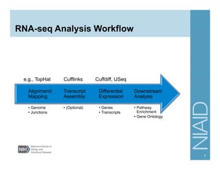
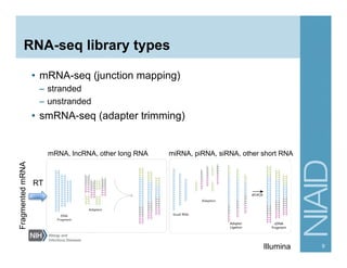
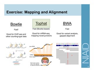
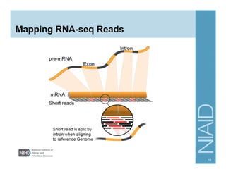
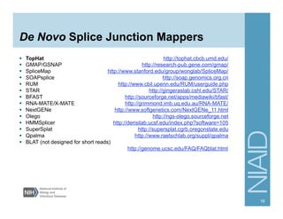
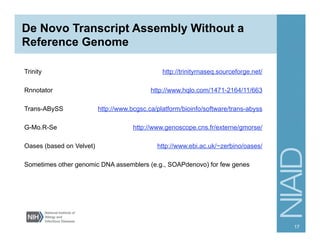
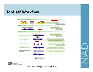
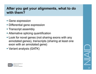
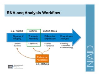
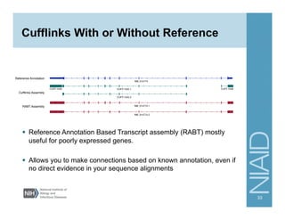
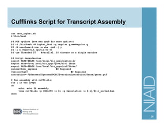
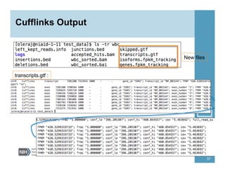
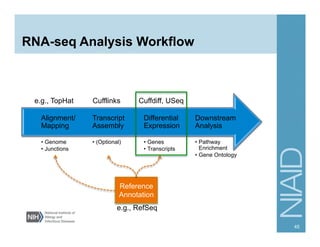
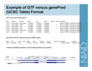
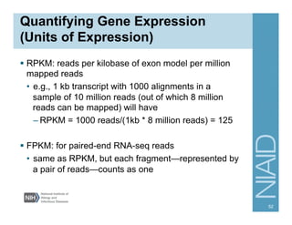
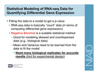
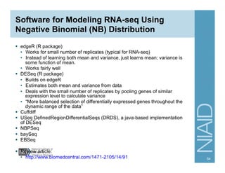
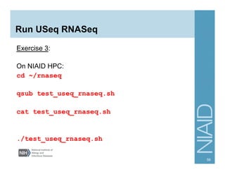
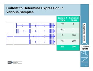
The document provides an overview of RNA sequencing (RNA-seq) analysis, including its advantages over traditional microarray methods, such as genome-wide coverage and reduced costs. It outlines the various steps in the RNA-seq workflow including read mapping with tools like Tophat2, transcript assembly with Cufflinks, and differential expression analysis. Additionally, the document describes library preparation protocols for different types of RNA and highlights the growing accessibility and cost-effectiveness of sequencing technologies.

1. Next Generation Sequencing Analysis Series
February 18, 2015
Andrew Oler, PhD
High-throughput Sequencing Bioinformatics Specialist
BCBB/OCICB/NIAID/NIH

2. Bioinformatics and Computational
Biosciences Branch
§ “BCBB”
§ Group of ~30
§ Bioinformatics Software
Developers
§ Computational Biologists
§ Project Managers &
Analysts
http://www.niaid.nih.gov/about/organization/odoffices/omo/ocicb/Pages/bcbb.aspx 2

3. The plan…
§ RNA-seq introduction
§ Mapping RNA-seq reads with TopHat2
§ Transcript assembly with Cufflinks
§ Differential expression
• USeq (DESeq2)
• Cuffdiff
3

4. Advantages of RNA-Seq
§ Genome-wide
• Unlike microarray where you look at selected regions
§ Doesn’t require existing genomic sequence
• Unlike microarray
§ Very low background noise
• Reads can be mapped with high confidence or tossed if poor quality
§ Resolution
• 1 bp, so you can look at variants, isoforms
§ High-throughput
• Much more sequence in a faster time compared to Sanger
§ Cost
• 1000X cheaper than Sanger sequencing
§ Drawbacks
• Depth of coverage depends on sequenceability (GC bias for PCR-based
amplification procedures)
4

5. Cost of Sequencing Has Dropped Exponentially
5
Sboner et al. Genome Biology 2011 12:125

6. RNA-seq Quantifies Accurate Gene
Expression Over a Large Linear Range
6
Range for RNA-seq expression quantification linear over 5 orders of magnitude

7. RNA-seq Analysis Workflow
• Pathway
Enrichment
• Gene Ontology
Downstream
Analysis
• Genes
• Transcripts
Differential
Expression
• (Optional)
Transcript
Assembly
• Genome
• Junctions
Alignment/
Mapping
7
e.g., TopHat Cufflinks Cuffdiff, USeq

8. RNA-seq Datasets in Public Short Read
Repositories
§ e.g., NIH/NCBI
• Short Read Archive (http://www.ncbi.nlm.nih.gov/sra)
• Gene Expression Omnibus (http://www.ncbi.nlm.nih.gov/geo/)
§ Human BodyMap 2.0 (Illumina)
• 16 normal tissues
• mRNA-seq 1x50 bp and 2x75 bp for each tissue
• Stranded mRNA-seq, total RNA stranded + DSN, mRNA stranded + DSN for
mixed tissues sample
• http://www.ensembl.info/blog/2011/05/24/human-bodymap-2-0-data-from-
illumina/
• http://tinyurl.com/hbm2data
• http://www.ebi.ac.uk/ena/data/view/ERP000546
8

9. RNA-seq library types
• mRNA-seq (junction mapping)
– stranded
– unstranded
• smRNA-seq (adapter trimming)
9
3
roduction
This protocol explains how to prepare libraries of chromatin-immuno-
precipitated DNA for analysis on the Illumina Cluster Station and Genome
Analyzer. You will add adapter sequences onto the ends of DNA fragments
to generate the following template format:
Figure 1 Fragments after Sample Preparation
The adapter sequences correspond to the two surface-bound oligos on
the flow cells used in the Cluster Station.
DNA
Fragment
Adapters
3
Introduction
This protocol explains how to prepare libraries of small RNA for subsequent
cDNA sequencing on the Illumina Cluster Station and Genome Analyzer.
You will physically isolate small RNA, ligate the adapters necessary for use
during cluster creation, and reverse-transcribe and PCR to generate the
following template format:
Figure 1 Fragments after Sample Preparation
The 5’ small RNA adapter is necessary for reverse transcription and
amplification of the small RNA fragment. This adapter also contains the DNA
sequencing primer binding site. The 3’ small RNA adapter corresponds to
the surface bound amplification primer on the flow cell used on the Cluster
Station.
Small RNA
Adapters
cDNA
Fragment
Adapter
Ligation
RT-PCR
Illumina
miRNA, piRNA, siRNA, other short RNA
mRNA, lncRNA, other long RNA
Fragmented
mRNA
RT

10. Exercise: Mapping and Alignment
10
Bowtie
Fast!
Good for ChIP-seq and
other counting-type data
Tophat
Fast (Bowtie-based)
Good for mRNA-seq,
mapping novel junctions
BWA
Fast
Good for variant analysis,
gapped alignment

11. Mapping RNA-seq Reads
11

12. Strategies for Mapping Junction Reads
§ Align to Transcriptome
• Create reference genome of all transcripts instead of genomic sequence
• Based on known splice sites
• No novel genes or transcripts
• Potential problem for alternative splice sites which causes repetition in the
reference, as well as conversion of coordinates back to reference
• e.g., any typical short read aligner
12
Align
reads to
transcripts

13. Strategies for Mapping Junction Reads
§ Splice Junction Sequences
• Construct sequence of all junctions, include with reference genomic sequence as
separate “chromosomes”
– e.g., use MakeSpliceJunctionFasta from USeq package
– http://useq.sourceforge.net/
• Based on known splice sites, no novels
• Need to convert coordinates back to reference
– USeq SamParser will do this for you
• e.g., ERANGE, or any typical short read aligner (after manually creating splice
junction sequences)
13
genomic
splice junctions

14. Strategies for Mapping Junction Reads
§ Split reads and align separately to reference
• Sometimes based on intermediate reference of reconstructed splice
junction sequences
• Finds known and novel splice sites
• e.g., TopHat, SOAPsplice
14
Frontiers in Genetics, Huang 2011

15. Strategies for Mapping Junction Reads
§ Allow large gaps in mapping
• Map as much of the read as possible, then take the
remaining sequence and find a nearby match for it.
• Finds known and novel splice sites
• e.g., STAR
• Requires lots of RAM (~30G for human)
15
?

16. De Novo Splice Junction Mappers
§ TopHat http://tophat.cbcb.umd.edu/
§ GMAP/GSNAP http://research-pub.gene.com/gmap/
§ SpliceMap http://www.stanford.edu/group/wonglab/SpliceMap/
§ SOAPsplice http://soap.genomics.org.cn
§ RUM http://www.cbil.upenn.edu/RUM/userguide.php
§ STAR http://gingeraslab.cshl.edu/STAR/
§ BFAST http://sourceforge.net/apps/mediawiki/bfast/
§ RNA-MATE/X-MATE http://grimmond.imb.uq.edu.au/RNA-MATE/
§ NextGENe http://www.softgenetics.com/NextGENe_11.html
§ Olego http://ngs-olego.sourceforge.net
§ HMMSplicer http://derisilab.ucsf.edu/index.php?software=105
§ SuperSplat http://supersplat.cgrb.oregonstate.edu
§ Qpalma http://www.raetschlab.org/suppl/qpalma
§ BLAT (not designed for short reads)
http://genome.ucsc.edu/FAQ/FAQblat.html
16

17. De Novo Transcript Assembly Without a
Reference Genome
17
Trinity http://trinityrnaseq.sourceforge.net/
Rnnotator http://www.hqlo.com/1471-2164/11/663
Trans-ABySS http://www.bcgsc.ca/platform/bioinfo/software/trans-abyss
G-Mo.R-Se http://www.genoscope.cns.fr/externe/gmorse/
Oases (based on Velvet) http://www.ebi.ac.uk/~zerbino/oases/
Sometimes other genomic DNA assemblers (e.g., SOAPdenovo) for few genes

18. TopHat
18

19. TopHat2 Workflow
19
Genome Biology, 2013, 14:R36

20. Tuxedo Workflow
§ October 2014 Protocol Paper:
§ http://www.nature.com/nprot/journal/v7/n3/full/nprot.
2012.016.html
20

21. TopHat2 Pre-requisites
§ http://ccb.jhu.edu/software/tophat/manual.shtml
§ Must be on PATH:
• bowtie2 and bowtie2-align (or bowtie)
• bowtie2-inspect (or bowtie-inspect)
• bowtie2-build (or bowtie-build)
• samtools
§ Python version 2.6 or higher
§ Install pre-compiled binary files, or compile from
source
21

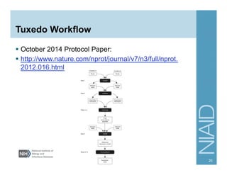
22. TopHat Command Line
22
tophat [options]* <index_base> <reads1_1> [reads1_2]
e.g., Paired-end
tophat hg19 SRR027894_1.fastq SRR027894_2.fastq
tophat hg19 SRR027894_1.fastq,SRR027895_1.fastq SRR027894_2.fastq,SRR027895_2.fastq
e.g., Single-end
tophat hg19 SRR036642.fastq
tophat hg19 SRR036642.fastq,SRR036643.fastq
Right mate in
paired-end
Single-end
or left mate in
paired-end
Index name
(genome)

23. TopHat Options
-o/--output-dir <string> Name of output directory. Default “./tophat_out”
-r <int> Mean inner distance between mate pairs = Mean fragment length -
( 2 * sequenced length). E.g., 250bp fragment, paired-end 100bp =>
-r 50 (default: 50)
--mate-std-dev <int> Standard deviation of distribution of inner distance (default: 20)
-N/--read-mismatches Number of mismatches allowed (default: 2)
--read-gap-length Total length of gaps allowed for a read (default: 2)
--read-edit-dist Total edit distance allowed (default: 2)
-a <int> Length required on both sides of junction (“anchor”) (default: 8).
-m <int> Maximum number of mismatches in anchor (default: 0)
-i <int> Minimum intron length (default: 70)
-I <int> Maximum intron length (default: 500000)
--solexa1.3-quals Illumina version 1.3-1.7 (phred+64)
-F <0.0-1.0> Minimum ratio of reads junction to exon reads to keep junction;
ensures junctions have good support (default: 0.15).
-p <int> Number of threads/processors (default: 1)
-g <int> Maximum number of alignments allowed (default: 20)
--microexon-search Attempt to find alignments around micro-exons
--library-type fr-unstranded, fr-firststrand, fr-secondstrand (for various library
types; see manual)
--segment-length Length to cut up reads for splice junction mapping (default: 25). For
36 bp reads, 18 bp is optimal.
-G GTF file containing genes (can get from UCSC Table Browser or
iGenomes) 23
http://tophat.cbcb.umd.edu/manual.html

24. TopHat Transcriptome Index Mode
§ If running multiple samples on the same index, first
create a transcriptome index:
tophat -G <GTF file> --transcriptome-
index <index base name>
<genome_index_base>
tophat -G hg19_refFlat.gtf --
transcriptome-index hg19_genes hg19
24

25. Running Tophat
Exercise 1:
On NIAID HPC:
qsub test_tophat.sh
On Helix:
./test_tophat.sh
Look at script:
cat test_tophat.sh
• Alignment
– tophat -o lymph -p 2 -G hg19_chr6_refFlat_noRandomHapUn.gtf chr6
lymph_aln.fastq.gz
– tophat -o wbc -p 2 -G hg19_chr6_refFlat_noRandomHapUn.gtf chr6
wbc_aln.fastq.gz
25
Demo TopHat interface, or save to the end to do all in a workflow?

26. TopHat Resume
§ If a TopHat job dies prematurely (e.g., killed by the
scheduler), you can resume from last successful
checkpoint
§ Just use the -R/--resume option followed by your
output directory (-o argument or tophat_out)
§ No other parameters necessary (they will be found in
the logs/run.log file)
tophat -R tophat_out
26

27. TopHat2 Output Files
accepted_hits.bam All read alignments
unmapped.bam Unmapped reads
junctions.bed Junction counts
align_summary Alignment summary stats
27

28. Post-Alignment Processing:
Transcript Assembly and
Annotation
28

29. After you get your alignments, what to do
with them?
§ Gene expression
§ Differential gene expression
§ Transcript assembly
§ Alternative splicing quantification
§ Look for novel genes (not sharing exons with any
annotated genes), transcripts (sharing at least one
exon with an annotated gene)
§ Variant analysis (GATK)
29

30. RNA-seq Analysis Workflow
• Pathway
Enrichment
• Gene Ontology
Downstream
Analysis
• Genes
• Transcripts
Differential
Expression
• (Optional)
Transcript
Assembly
• Genome
• Junctions
Alignment/
Mapping
30
Reference
Annotation
e.g., TopHat Cufflinks
e.g., RefSeq
Cuffdiff, USeq

31. Transcript Assembly Software
§ Map reads to junctions
§ Build connectivity graph
§ Determine significant segments
§ Example software:
• Cufflinks
• Scripture
• Inchworm
• IsoLasso
31
[#%>)AT)K4%(FON)97%5:%(#7<)"-&677)#$%)5&">$)
[#%>)CT)3'(4)7'5('V-"(#)7%5:%(#7)
Statistical reconstruction of the transcriptome
Manuel Garber

32. Cufflinks Overview
32
Cufflinks assembles transcripts based
largely on spliced reads, and estimates
abundances of each isoform of a gene

33. Cufflinks With or Without Reference
§ Reference Annotation Based Transcript assembly (RABT) mostly
useful for poorly expressed genes.
§ Allows you to make connections based on known annotation, even if
no direct evidence in your sequence alignments
33
Reference Annotation
Cufflinks Assembly
RABT Assembly
NM_014774.2
NM_014774.1
CUFF.1545.1
CUFF.1540
NM_014774
CUFF.1546
CUFF.1545.2
Fig. 3. Comparison of assembler output for an example gene. Lack of sequencing coverage in the UTR and across one splice junction caused the Cufflinks
ssembler (teal) to output three transfrags that match the reference (blue) and a fourth that contains a novel splice junction. The RABT assembler output
red) includes both the reference transcript (NM 014774.1) and a novel isoform (NM 014774.2) that is assembled from a combination of sequencing reads,
which reveal the novel junction, and faux-reads, which connect the three sections to form a single transcript. Note that even with the addition of the reference
ranscript, the total number of transfrags output by the assembler has been reduced for this locus, and the transfrag lengths have increased.
D. melanogaster Output Set # of Genes # of Transfrags Avg Transfrag Length Isoforms Per Gene
Reference Annotation 13,302 20,715 1,629 1.56
Cufflinks Assembly 7,167 8,701 2,334 1.21
Cufflinks Assembly (Novel Only) 350 3,205 2,741 -
RABT Assembly 13,634 23,913 1,815 1.75
RABT Assembly (Novel Only) 332 3,018 2,719 -
Table 2. Results for two different versions of assembly on the first Drosophila melanogaster embryo time-point from (Graveley et al., 2010). The categories
an be interpreted in the same manner as Table 1. These results show that the method also produces improved assemblies in fly.
http://bioinforma
Downloaded
from

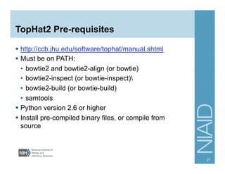
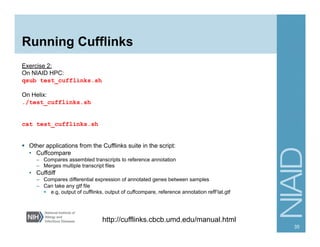
34. Cufflinks Options
cufflinks [options]* <aligned_reads.(sam/bam)>
Options:
-o output directory
-p number of threads/processors (default: 1)
-G <path> Use GTF/GFF annotation file to use determine isoform
expression. Do not assemble novel transcripts.
-g <path> Use GTF/GFF to guide assembly of annotated transcripts
(RABT); also assembly novel genes and isoforms
-M <path> GTF/GFF file containing regions to exclude from analysis, e.g.,
chrM, rRNA
-b <genome.fa> perform bias correction
-u multi-read correction calculation
--library-type <str> fr-unstranded (default), fr-firststrand (dUTP method), fr-
secondstrand (directional Illumina)
-F <0.0-1.0> minimum isoform fraction to include an isoform. (default: 0.1,
which means at least 10% of the most abundant isoform of the
gene)
Command:
cufflinks -o cuff_out -p 5 -g hg19_refFlat.gtf -M chrM_rRNA.gtf
-u -b genome.fa accepted_hits.bam
34
http://cufflinks.cbcb.umd.edu/manual.html

35. Running Cufflinks
Exercise 2:
On NIAID HPC:
qsub test_cufflinks.sh
On Helix:
./test_cufflinks.sh
cat test_cufflinks.sh
§ Other applications from the Cufflinks suite in the script:
• Cuffcompare
– Compares assembled transcripts to reference annotation
– Merges multiple transcript files
• Cuffdiff
– Compares differential expression of annotated genes between samples
– Can take any gtf file
§ e.g, output of cufflinks, output of cuffcompare, reference annotation refFlat.gtf
35
http://cufflinks.cbcb.umd.edu/manual.html

36. Cufflinks Script for Transcript Assembly
cat test_tophat.sh
#!/bin/bash
## SGE options (see man qsub for more options)
#$ -S /bin/bash -N tophat_test -q regular.q,memRegular.q
#$ -M user@email.com -m abe -cwd -j y
#$ -l h_vmem=7G,h_cpu=12:00:00
#$ -pe threaded 10 #Parallel, 10 threads on a single machine
## Script dependencies
export PATH=$PATH:/usr/local/bio_apps/samtools/
export PATH=/usr/local/bio_apps/java/bin/:$PATH
export PATH=$PATH:/usr/local/bio_apps/cufflinks/
genome=Homo_sapiens ## Required
version=hg19 ## Required
annotation=~/iGenomes/$genome/UCSC/$version/Annotation/Genes/genes.gtf
# Run assembly with cufflinks:
for i in wbc lymph
do
echo; echo $i assembly
time cufflinks -p $NSLOTS -o $i -g $annotation -u ${i}/${i}_sorted.bam
done
36

37. Cufflinks Output
37
New files
transcripts.gtf :

38. Cufflinks Output
38
isoforms.fpkm_tracking :
genes.fpkm_tracking :

39. Cuffcompare to Compare Transcripts to
Reference and Merge from Multiple Samples
39
Reference:
Sample 1:
Sample 2:
Merged:
In merged table, genes (XLOC) and transcripts (TCONS) are renamed.
Hint: -R will allow you to ignore any reference transcripts not present in your sample.
http://cufflinks.cbcb.umd.edu/manual.html#cuffcompare

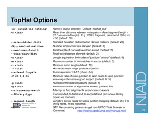
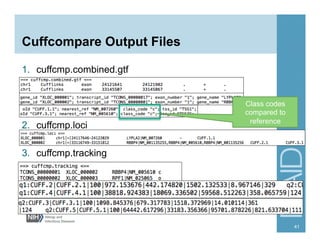
40. Running Cuffcompare
cuffcompare [options] <transcripts1.gtf>
<transcripts2.gtf> …
e.g.,
cuffcompare -r hg19_chr6_refFlat_noRandomHapUn.gtf
lymph/transcripts.gtf wbc/transcripts.gtf
-r [file] Reference transcripts in gtf format
-R Ignore reference transcripts not found in
RNAseq sample
40

41. Cuffcompare Output Files
1. cuffcmp.combined.gtf
2. cuffcmp.loci
3. cuffcmp.tracking
41
Class codes
compared to
reference

42. Cufflinks (Cuffcompare) Class Codes
42

43. Transcript Assembly Conclusion
§ RNA-seq reads can be processed to determine all
of the transcripts expressed in a tissue.
§ Important parameters for RNA-seq library prep if
transcript assembly is a goal are
• long reads (50 bp, 75 bp, 100 bp …)
• stranded could help…
• paired-end reads help
§ RABT is good for genes with low expression…
§ Be aware that all of the reference transcripts will
be in the output if you use RABT.
§ Cuffcompare can be used to compare expressed
transcripts to a reference annotation
43

44. Post-Alignment Processing:
Gene Expression
44

45. RNA-seq Analysis Workflow
• Pathway
Enrichment
• Gene Ontology
Downstream
Analysis
• Genes
• Transcripts
Differential
Expression
• (Optional)
Transcript
Assembly
• Genome
• Junctions
Alignment/
Mapping
45
Reference
Annotation
e.g., TopHat Cufflinks
e.g., RefSeq
Cuffdiff, USeq

46. Using RNA-seq Data to Quantify Gene
Expression
§ Goals:
1. Determine which genes are expressed in a tissue
a. Catalogue of genes expressed above a certain level
b. List of the top X number of expressed genes
2. Determine differential expression of genes
a. Between two different tissues
b. Between two samples treated differently
1) treatment versus control
3. Determine differential post-transcriptional regulation of genes
a. Differential splicing between two samples
b. Differential RNA editing
c. Differential translation (ribosomal profiling)
46
Treatment
Changes in
Gene
Expression
Phenotype
?

47. Gene Models
47

48. Gene Model Prediction Databases
§ NCBI RefSeq (http://www.ncbi.nlm.nih.gov/RefSeq/)
§ Ensembl (www.ensembl.org)
§ Mammalian Gene Collection (http://mgc.nci.nih.gov/)
§ UCSC Known Genes(http://genome.ucsc.edu/cgi-bin/hgTables)
§ Vega (http://vega.sanger.ac.uk/)
§ AceView (http://www.ncbi.nlm.nih.gov/IEB/Research/Acembly/)
48

49. Gene Annotation Files
§ Formats
• One line per feature (e.g., exon, transcript, etc.)
– GFF3 (most widely used; the standard)
– GTF (UCSC, TopHat, Cufflinks)
• One line per gene (e.g., all exon starts and stops one line)
– UCSC gene table (UCSC, USeq)
– BED12 (BEDtools)
§ Where to Download Annotation for your Genome
• UCSC Table Browser (http://genome.ucsc.edu/cgi-bin/hgTables)
• BioMart (http://www.biomart.org/)
• iGenomes (http://tophat.cbcb.umd.edu/igenomes.html)
ls /gpfs/bio_data/iGenomes/Homo_sapiens/UCSC/hg19/Annotation/Genes/
ChromInfo.txt
cytoBand.txt
genes.gtf
kgXref.txt
knownGene.txt
refFlat.txt
refGene.txt
knownToRefSeq.txt
refMrna.fa
refSeqSummary.txt
49
GTF format
UCSC Table/genePred format

50. UCSC Table Browser
http://genome.ucsc.edu/
50
Refseq
Ensembl
UCSC KnownGene
Vega
AceView

51. Example of GTF versus genePred
(UCSC Table) Format
GTF record for PRM1 gene:
#chr source feature start end score strand frame attributes
chr16 hg19_refFlat stop_codon 11374849 11374851 0.000000 - . gene_id "PRM1"; transcript_id "PRM1";
chr16 hg19_refFlat CDS 11374852 11374892 0.000000 - 2 gene_id "PRM1"; transcript_id "PRM1";
chr16 hg19_refFlat exon 11374693 11374892 0.000000 - . gene_id "PRM1"; transcript_id "PRM1";
chr16 hg19_refFlat CDS 11374984 11375095 0.000000 - 0 gene_id "PRM1"; transcript_id "PRM1";
chr16 hg19_refFlat start_codon 11375093 11375095 0.000000 - . gene_id "PRM1"; transcript_id "PRM1";
chr16 hg19_refFlat exon 11374984 11375192 0.000000 - . gene_id "PRM1"; transcript_id "PRM1";
genePred (UCSC Table) record for PRM1 gene:
#gene name chrom strand txStart txEnd cdsStart cdsEnd exonCount exonStarts exonEnds
PRM1 NM_002761 chr16 - 11374692 11375192 11374848 11375095 2 11374692,11374983, 11374892,11375192,
*TopHat and Cufflinks applications use GTF, USeq applications use genePred.
51

52. Quantifying Gene Expression
(Units of Expression)
§ RPKM: reads per kilobase of exon model per million
mapped reads
• e.g., 1 kb transcript with 1000 alignments in a
sample of 10 million reads (out of which 8 million
reads can be mapped) will have
– RPKM = 1000 reads/(1kb * 8 million reads) = 125
§ FPKM: for paired-end RNA-seq reads
• same as RPKM, but each fragment—represented by
a pair of reads—counts as one
52

53. Statistical Modeling of RNA-seq Data for
Quantifying Differential Gene Expression
§ Fitting the data to a model to get a p-value
• RNA-seq data is basically “count” data (in terms of
computing differential gene expression)
• Negative Binomial is a suitable statistical method
– Good for modeling skewed and overdispersed
data (e.g., biological data)
– Mean and Variance need to be learned from the
data to fit the model
§ Need many biological replicates for accurate
results (hint for experimental design)
53

54. Software for Modeling RNA-seq Using
Negative Binomial (NB) Distribution
§ edgeR (R package)
• Works for small number of replicates (typical for RNA-seq)
• Instead of learning both mean and variance, just learns mean; variance is
some function of mean.
• Works fairly well
§ DESeq (R package)
• Builds on edgeR
• Estimates both mean and variance from data
• Deals with the small number of replicates by pooling genes of similar
expression level to calculate variance
• “More balanced selection of differentially expressed genes throughout the
dynamic range of the data”
§ Cuffdiff
§ USeq DefinedRegionDifferentialSeqs (DRDS), a java-based implementation
of DESeq
§ NBPSeq
§ baySeq
§ EBSeq
§ Review article:
• http://www.biomedcentral.com/1471-2105/14/91 54

55. Negative Binomial Models the Variance of
the Data With Respect to the Mean
55
Anders and Huber Genome Biology 2010 11:R106 doi:10.1186/gb-2010-11-10-r106
Purple = Poisson Orange solid = DESeq Orange dotted = edgeR

56. USeq Package Programs for Differential
RNA-seq Analysis
§ DefinedRegionDifferentialSeq
§ RNASeq (wrapper)
– Converts splice junction coordinates to genomic coordinates
(important when aligning to genome+junctions index)
– Computes Read depth coverage plots for visualization in IGB
– Pairwise differential expression between all samples using DESeq.
– Identification of novel transfrags with differential expression
between samples.
§ Documentation/Usage:
• Extended Splice Junction RNA-seq Analysis
(http://useq.sourceforge.net/usageRNASeq.html)
56
http://useq.sourceforge.net/usage.html
http://useq.sourceforge.net/applications.html

57. Gene or Transcript Expression?
57
Transcripts/Isoforms:
Flattened Gene (all possible exon space):

58. USeq DefinedRegionDifferentialSeq for
Differential Expression Analysis
§ Calculate expression value as Fragments Per Kilobase of exon
model per Million mapped reads (FPKM)
§ Calculate p-value and false discovery rate (FDR) for differential
expression using DESeq2 and
Options
-s <path> Output directory for saving results
-c <path> Directory containing alignments. Separate directory
for each condition.
-u <path> UCSC RefFlat gene table (genePred format)
-r <path> Full path to R containing DESeq2
-g <string> Genome version (e.g., H_sapiens_Feb_2009)
Command:
java -Xmx1G -jar /usr/local/bio_apps/USeq/Apps/DefinedRegionDifferentialSeq
-s output -c alignments -u hg19_refFlat_chr6_part_Merged.ucsc
-r /usr/local/bio_apps/R/bin/R -g H_sapiens_Feb_2009
58

59. Run USeq RNASeq
Exercise 3:
On NIAID HPC:
cd ~/rnaseq
qsub test_useq_rnaseq.sh
cat test_useq_rnaseq.sh
./test_useq_rnaseq.sh
59

60. Cuffdiff Workflow
60
http://cole-trapnell-lab.github.io/cufflinks/manual/
BAM BAM
GTF

61. Cuffdiff to Determine Expression In
Various Samples
61
Sample 1
FPKM
Sample 2
FPKM
10 5
600 1
2 100
15 200
627 306 2. Gene
FPKM
1.
Isoforms
FPKM

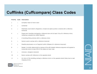
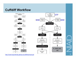
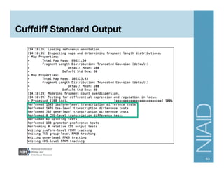
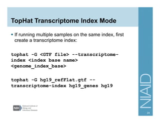
62. Running Cuffdiff
cuffdiff [options] <transcripts.gtf> <sample1.bam>
<sample2.bam> …
e.g.,
cuffdiff -p 10 cuffcmp.combined.gtf lymph/
accepted_hits.bam wbc/accepted_hits.bam
-p [INT] Number of processors
-o Output directory (default = current dir)
-T Treat samples as a time series (default =
all against all comparison)
-u Multi-read correction for reads that map
to multiple places in the genome
Others (type “cuffdiff” to see other options)
62

63. Cuffdiff Standard Output
63

64. Cuffdiff Output Files
1. cds.diff
2. promoters.diff
3. splicing.diff
4. cds_exp.diff
5. gene_exp.diff
6. tss_group_exp.diff
7. isoform_exp.diff
64
gene_exp.diff :
isoform_exp.diff :
sample 1: 96696 + 28223 + 45417.4 = 170336
sample 2: 37915.2 + 11160.4 + 0 = 49075.6
Copy and Paste
into Browser

65. CummeRbund
– CummeRbund takes the various output files from a cuffdiff run and
creates a SQLite database of the results describing appropriate
relationships betweeen genes, transcripts, transcription start sites, and
CDS regions.
– From there, you can create publication-quality figures to describe the
data.
65
http://compbio.mit.edu/cummeRbund/

66. Alternative Splicing Quantification
§ Mixture of Isoforms (MISO) + Sashimi plot
§ Splicing Analysis Kit (Spanki)
§ Multivariate Analysis of Transcript Splicing (MATS)
§ Cuffdiff
66
http://miso.readthedocs.org/en/fastmiso/

67. Other Demonstrations (Time-permitting)
§ Visualization of output in Genome Browsers
• IGB
• IGV
• Links to BAM files
– https://dl.dropbox.com/u/30379708/Upenn/
lymph_accepted_hits.bam
– https://dl.dropbox.com/u/30379708/Upenn/
wbc_accepted_hits.bam
§ GO Miner or DAVID
67

68. Downstream analysis
§ Goal is to determine
• What *types* of genes show a change in expression
• What cellular pathways are activated/inactivated by
your treatment
§ Software/websites:
• GO Miner
– http://discover.nci.nih.gov/gominer/
GoCommandWebInterface.jsp
• DAVID
– http://david.abcc.ncifcrf.gov/
• Ingenuity Pathway Analysis (IPA)
– http://www.ingenuity.com/products/pathways_analysis.html
68

69. Other Resources
§ RNA-seq tutorials
• https://sites.google.com/site/princetonhtseq/tutorials/rna-seq
• https://docs.uabgrid.uab.edu/wiki/
UAB_Galaxy_RNA_Seq_Step_by_Step_Tutorial
• http://en.wikibooks.org/wiki/Next_Generation_Sequencing_(NGS)/RNA
• https://main.g2.bx.psu.edu/
• http://useq.sourceforge.net/usage.html
• http://www.rna-seqblog.com/
• http://en.wikipedia.org/wiki/RNA-Seq
• http://link.springer.com/protocol/10.1007/978-1-61779-839-9_16/
fulltext.html
§ Commercial Software for RNA-seq Analysis (No Command Line!)
• Partek Genomics Suite
– http://www.partek.com/?q=partekgs
• CLCBio Genomics Workbench
– http://www.clcbio.com/products/clc-genomics-workbench/
69

70. Thank You
For questions or comments please contact:
andrew.oler@nih.gov
ScienceApps@niaid.nih.gov
70