The document provides an overview of linear regression and its components, such as least squares, matrix notation, and computation methods for large datasets. It discusses the conjugate gradient method as a solution for large matrices, the importance of regularization to avoid issues with linearly dependent features, and provides code snippets and statistical views to improve understanding and performance of regression models. Concepts like the maximum likelihood estimator, variance, and r-squared statistics are also highlighted, emphasizing the computational and theoretical aspects of linear regression.
![Computation of XTX
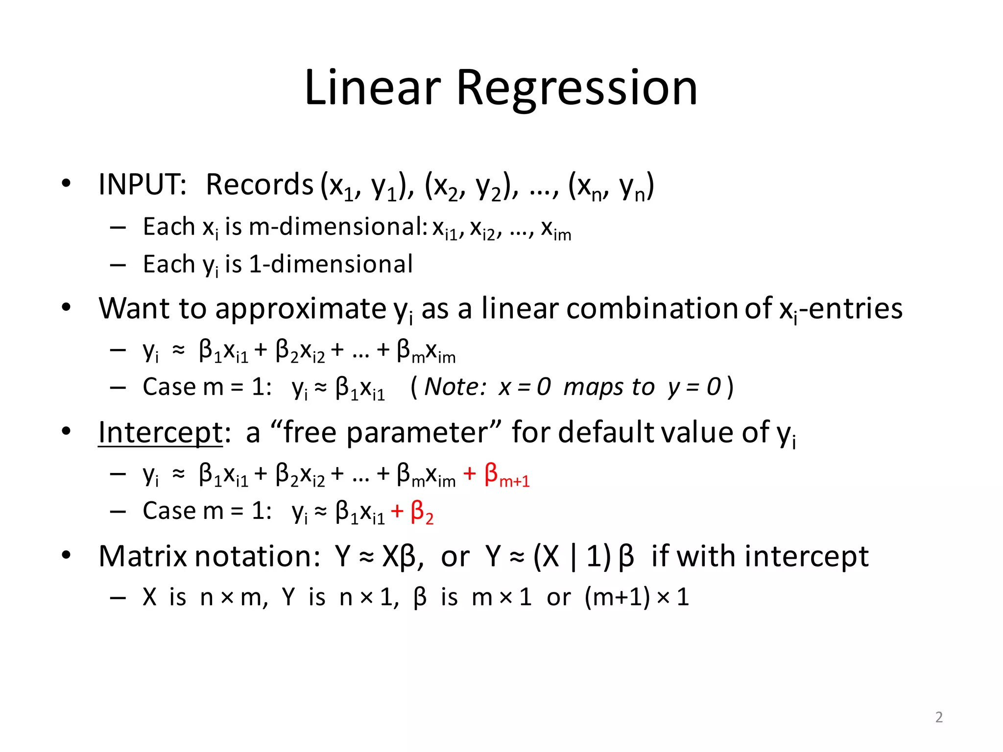
• Input (n × m)-matrix X is often huge and sparse
– Rows X[i, ] make up n records, often n >> 106
– Columns X[, j] are the features
• Matrix XTX is (m × m) and dense
– Cells: (XTX) [j1, j2] = ∑ i≤n X[i, j1] * X[i, j2]
– Part of covariance between features # j1 and # j2 across all records
– m could be small or large
• If m ≤ 1000, XTX is small and “direct solve” is efficient…
– … as long as XTX is computed the right way!
– … and as long as XTX is invertible (no linearly dependent features)
5](https://image.slidesharecdn.com/s3regressionlesson-160913183002/75/Regression-using-Apache-SystemML-by-Alexandre-V-Evfimievski-5-2048.jpg)
![Computation of XTX
• Naïve computation:
a) Read X into memory
b) Copy it and rearrange cells into the transpose
c) Multiply two huge matrices, XT and X
• There is a better way: XTX = ∑i≤n X[i, ]T X[i, ] (outer product)
– For all i = 1, …, n in parallel:
a) Read one row X[i, ]
b) Compute (m × m)-matrix: Mi [j1, j2] = X[i, j1] * X[i, j2]
c) Aggregate: M = M + Mi
• Extends to (XTX) v and XT diag(w) X, used in other scripts:
– (XTX) v = ∑i≤n (∑ j≤m X[i, j]v[j]) * X[i, ]T
– XT diag(w)X = ∑ i≤n wi * X[i, ]T X[i, ]
6](https://image.slidesharecdn.com/s3regressionlesson-160913183002/75/Regression-using-Apache-SystemML-by-Alexandre-V-Evfimievski-6-2048.jpg)
![Shifting and Scaling X
• PROBLEM: Features have vastly different range:
– Examples: [0, 1]; [2010, 2015]; [$0.01, $1 Billion]
• Each βi in Y ≈ Xβ has different size & accuracy?
– Regularization λ·βT β also range-dependent?
• SOLUTION: Scale & shift features to mean = 0, variance = 1
– Needs intercept: Y ≈ (X| 1)β
– Equivalently: (Xnew |1) = (X |1) %*% SST “Shift-Scale Transform”
• BUT: Sparse X becomes Dense Xnew …
• SOLUTION: (Xnew |1) %*% M = (X |1) %*% (SST %*% M)
– Extends to XTX and other X-products
– Further optimization: SST has special shape
11](https://image.slidesharecdn.com/s3regressionlesson-160913183002/75/Regression-using-Apache-SystemML-by-Alexandre-V-Evfimievski-11-2048.jpg)
![Shifting and Scaling X
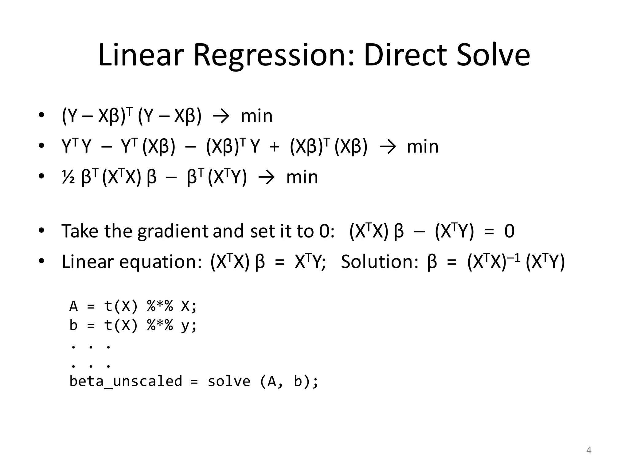
– Linear Regression Direct Solve
code snippet example:
A = t(X) %*% X;
b = t(X) %*% y;
if (intercept_status == 2) {
A = t(diag (scale_X) %*% A + shift_X %*% A [m_ext, ]);
A = diag (scale_X) %*% A + shift_X %*% A [m_ext, ];
b = diag (scale_X) %*% b + shift_X %*% b [m_ext, ];
}
A = A + diag (lambda);
beta_unscaled = solve (A, b);
if (intercept_status == 2) {
beta = scale_X * beta_unscaled;
beta [m_ext, ] = beta [m_ext, ] + t(shift_X) %*% beta_unscaled;
} else {
beta = beta_unscaled;
}
12](https://image.slidesharecdn.com/s3regressionlesson-160913183002/75/Regression-using-Apache-SystemML-by-Alexandre-V-Evfimievski-12-2048.jpg)
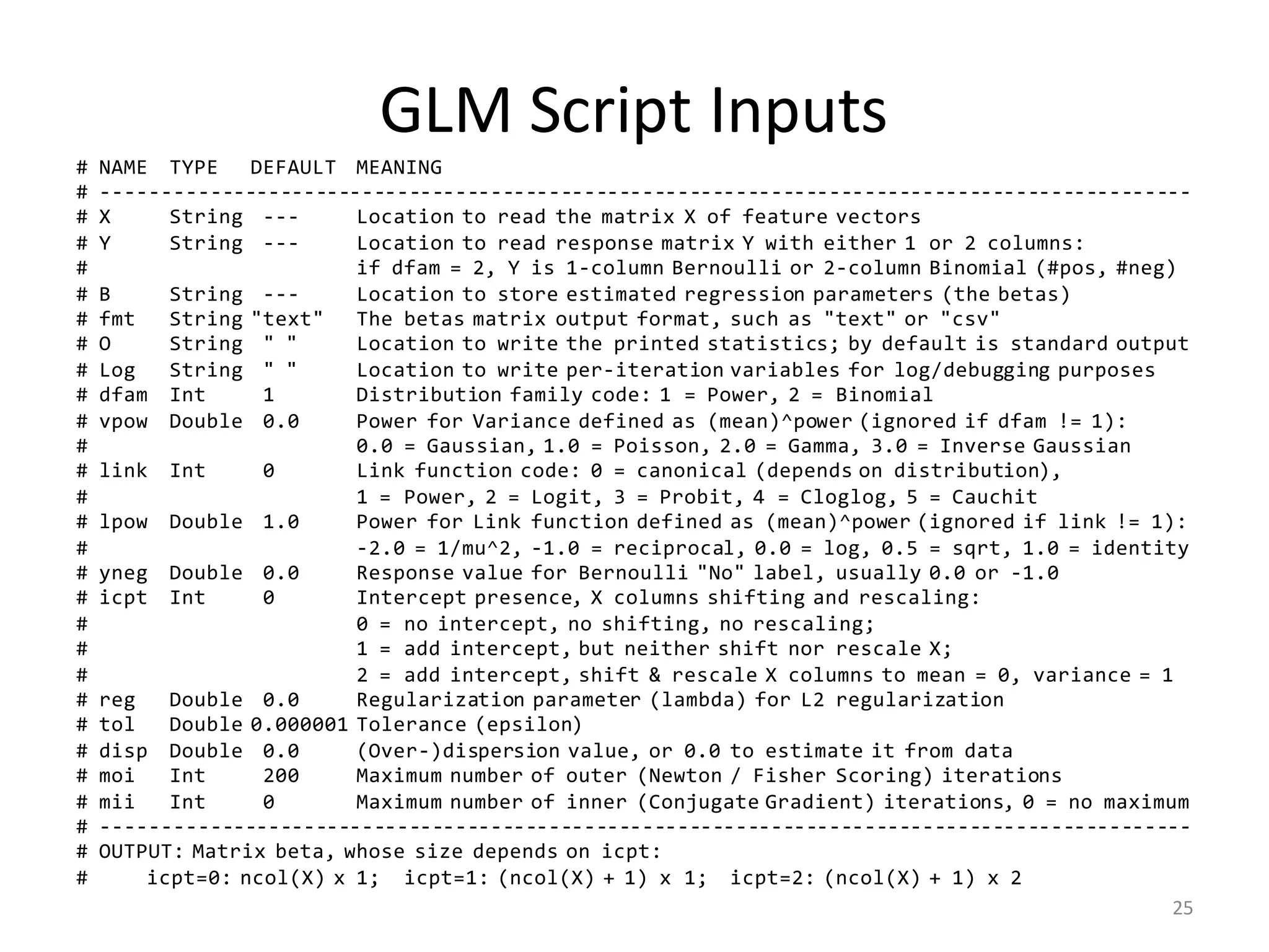
![LinReg Scripts: Inputs
# INPUT PARAMETERS:
# --------------------------------------------------------------------------------------------
# NAME TYPE DEFAULT MEANING
# --------------------------------------------------------------------------------------------
# X String --- Location (on HDFS) to read the matrix X of feature vectors
# Y String --- Location (on HDFS) to read the 1-column matrix Y of response values
# B String --- Location to store estimated regression parameters (the betas)
# O String " " Location to write the printed statistics; by default is standard output
# Log String " " Location to write per-iteration variables for log/debugging purposes
# icpt Int 0 Intercept presence, shifting and rescaling the columns of X:
# 0 = no intercept, no shifting, no rescaling;
# 1 = add intercept, but neither shift nor rescale X;
# 2 = add intercept, shift & rescale X columns to mean = 0, variance = 1
# reg Double 0.000001 Regularization constant (lambda) for L2-regularization; set to nonzero
# for highly dependend/sparse/numerous features
# tol Double 0.000001 Tolerance (epsilon); conjugate graduent procedure terminates early if
# L2 norm of the beta-residual is less than tolerance * its initial norm
# maxi Int 0 Maximum number of conjugate gradient iterations, 0 = no maximum
# fmt String "text" Matrix output format for B (the betas) only, usually "text" or "csv"
# --------------------------------------------------------------------------------------------
# OUTPUT: Matrix of regression parameters (the betas) and its size depend on icpt input value:
# OUTPUT SIZE: OUTPUT CONTENTS: HOW TO PREDICT Y FROM X AND B:
# icpt=0: ncol(X) x 1 Betas for X only Y ~ X %*% B[1:ncol(X), 1], or just X %*% B
# icpt=1: ncol(X)+1 x 1 Betas for X and intercept Y ~ X %*% B[1:ncol(X), 1] + B[ncol(X)+1, 1]
# icpt=2: ncol(X)+1 x 2 Col.1: betas for X & intercept Y ~ X %*% B[1:ncol(X), 1] + B[ncol(X)+1, 1]
# Col.2: betas for shifted/rescaled X and intercept
17](https://image.slidesharecdn.com/s3regressionlesson-160913183002/75/Regression-using-Apache-SystemML-by-Alexandre-V-Evfimievski-17-2048.jpg)
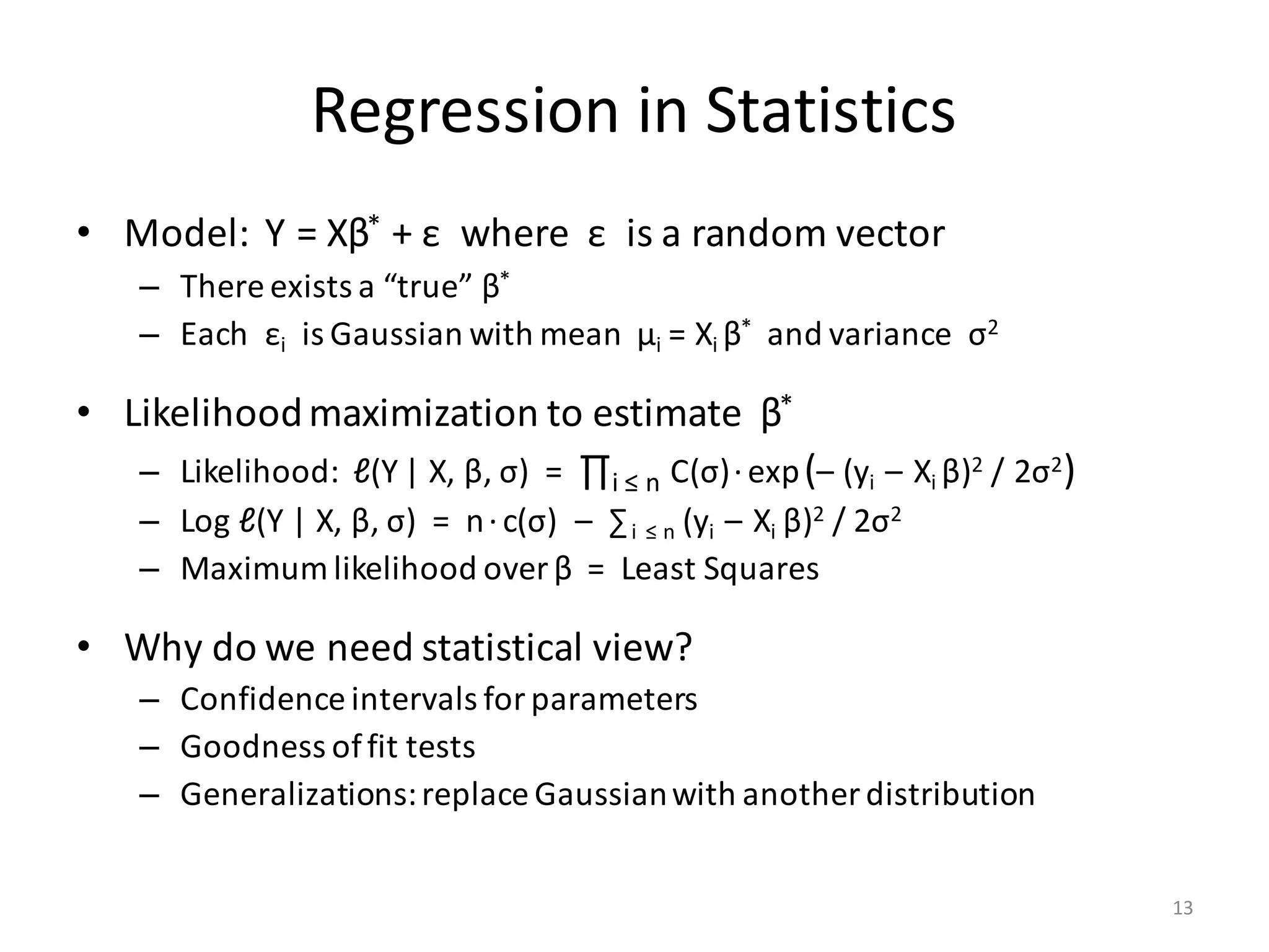
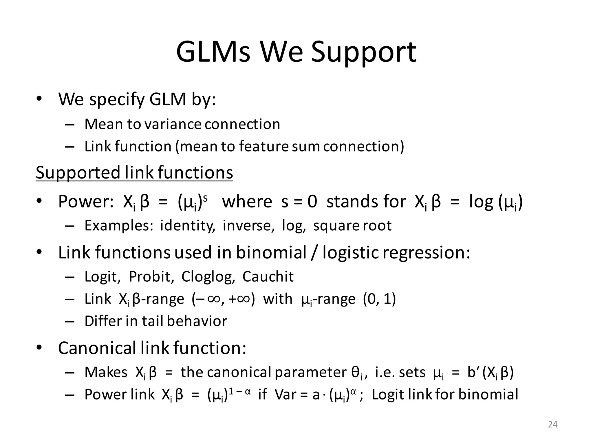
![Generalized Linear Models
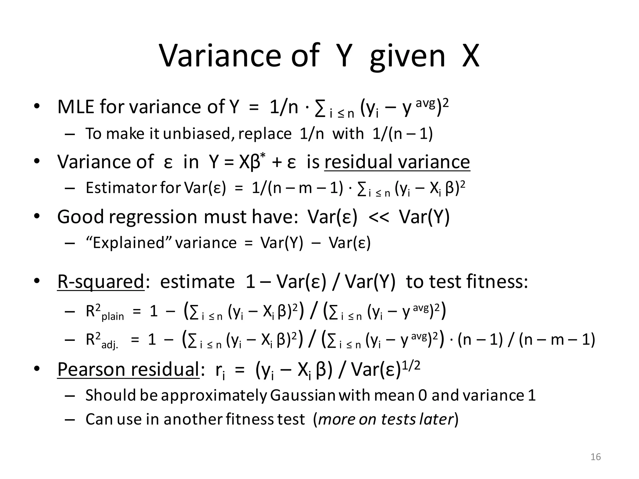
• Linear Regression: Y = Xβ* + ε
– Each yi is Normal(μi , σ2) where mean μi = Xi β*
– Variance(yi) = σ2 = constant
• Logistic Regression:
– Each yi is Bernoulli(μi) where mean μi = 1 / (1 + exp (– Xi β*))
– Prob [yi = 1] = μi , Prob [yi = 0] = 1 – μi , mean = probability of 1
– Variance(yi) = μi (1 – μi)
• Poisson Regression:
– Each yi is Poisson(μi) where mean μi = exp(Xi β*)
– Prob [yi = k] = (μi)k exp(– μi)/ k! for k = 0, 1, 2, …
– Variance(yi) = μi
• Only in Linear Regression we add error εi to mean μi
20](https://image.slidesharecdn.com/s3regressionlesson-160913183002/75/Regression-using-Apache-SystemML-by-Alexandre-V-Evfimievski-20-2048.jpg)
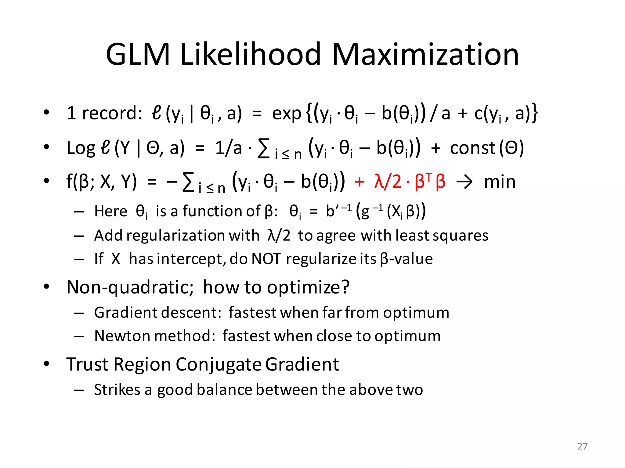
![Generalized Linear Models
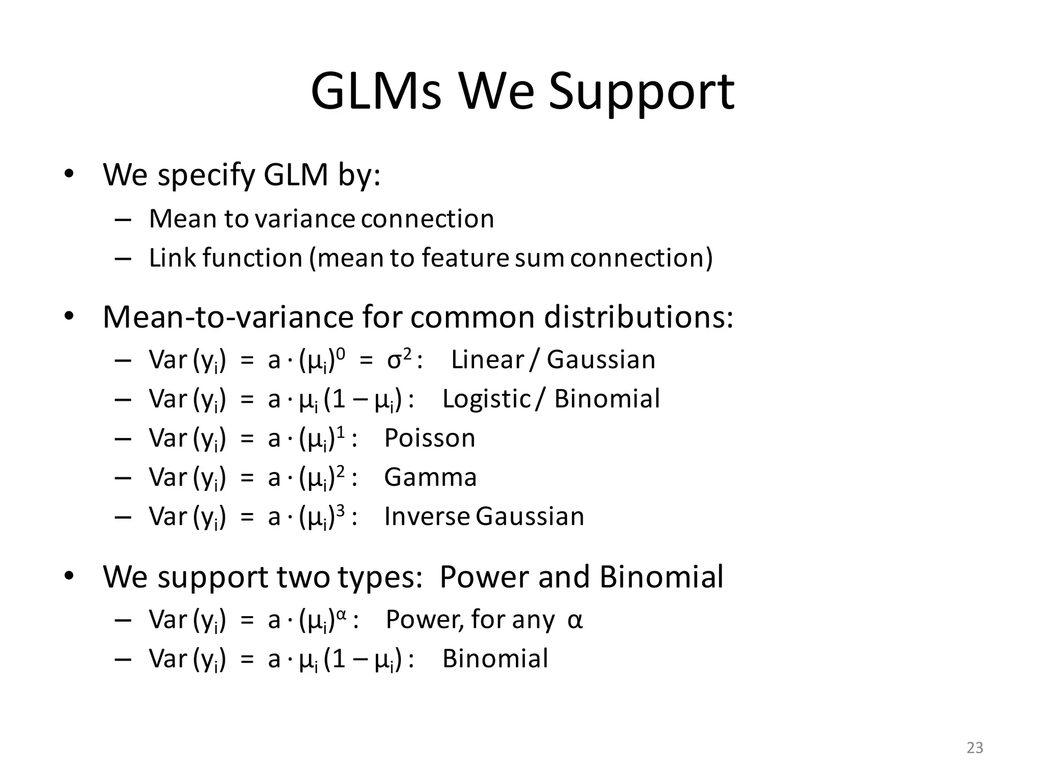
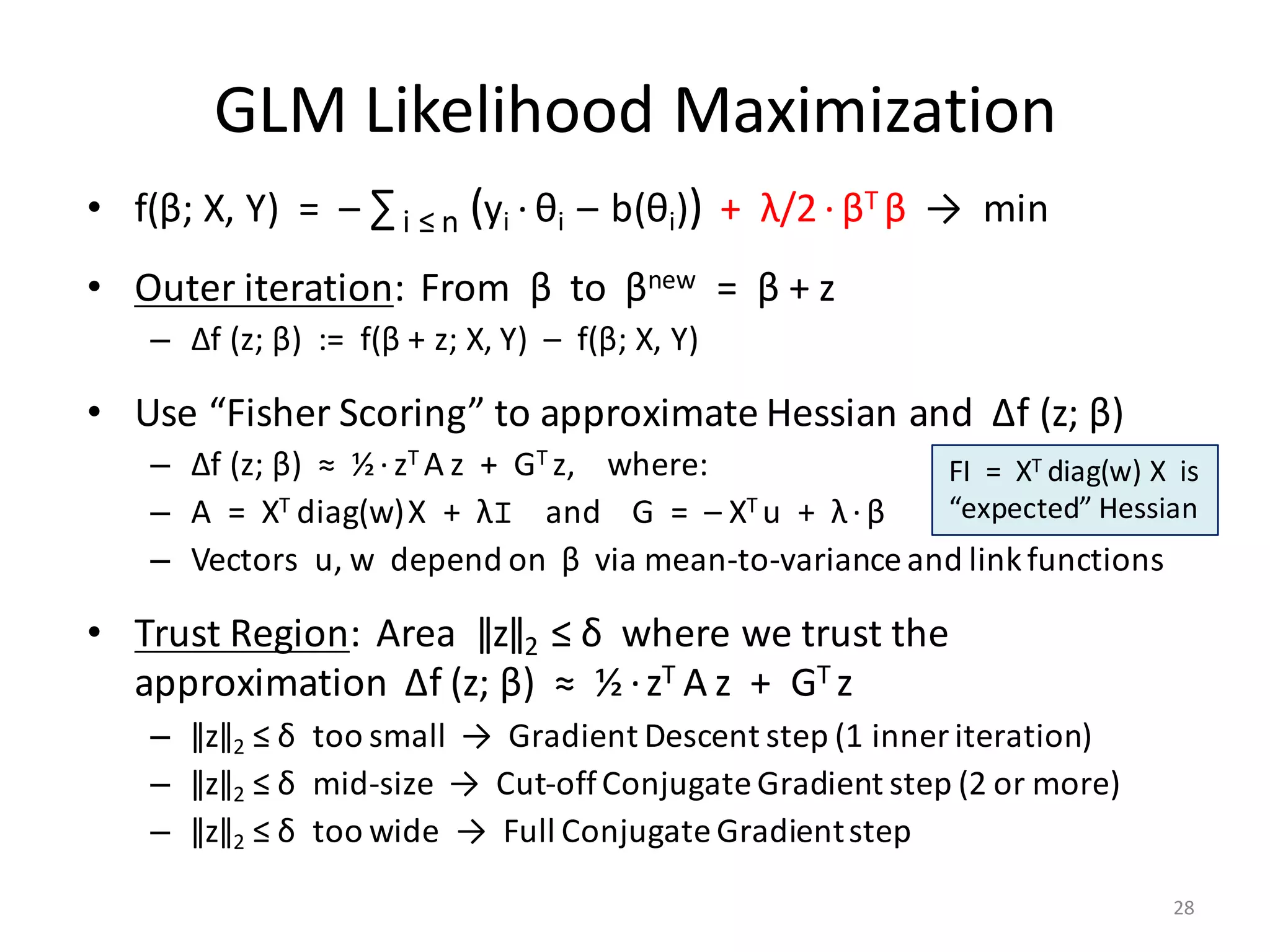
• GLM Regression:
– Each yi has distribution = exp{(yi ·θi – b(θi))/a + c(yi , a)}
– Canonical parameter θi represents the mean: μi = bʹ(θi)
– Link function connects μi and Xi β* : Xi β* = g(μi), μi = g –1 (Xi β*)
– Variance(yi) = a ·bʺ(θi)
• Example: Linear Regression as GLM
– C(σ)·exp(– (yi – Xi β)2 / 2σ2) = exp{(yi ·θi – b(θi))/a + c(yi , a)}
– θi = μi = Xi β; b(θi) = (Xi β)2 / 2; a = σ2 = variance
• Link function = identity; c(yi , a) = – yi
2 /2σ2 + log C(σ)
• Example: Logistic Regression as GLM
– (μi )y[i] (1 – μi)1 – y[i] = exp{yi · log(μi) – yi · log(1 – μi) + log(1 – μi)}
= exp{(yi ·θi – b(θi))/ a + c(yi , a)}
– θi = log(μi / (1 – μi)) = Xi β; b(θi) = – log(1 – μi) = log(1 + exp(θi))
• Link function = log (μ / (1 – μ)) ; Variance = μ(1 – μ) ; a = 1
21](https://image.slidesharecdn.com/s3regressionlesson-160913183002/75/Regression-using-Apache-SystemML-by-Alexandre-V-Evfimievski-21-2048.jpg)
![Generalized Linear Models
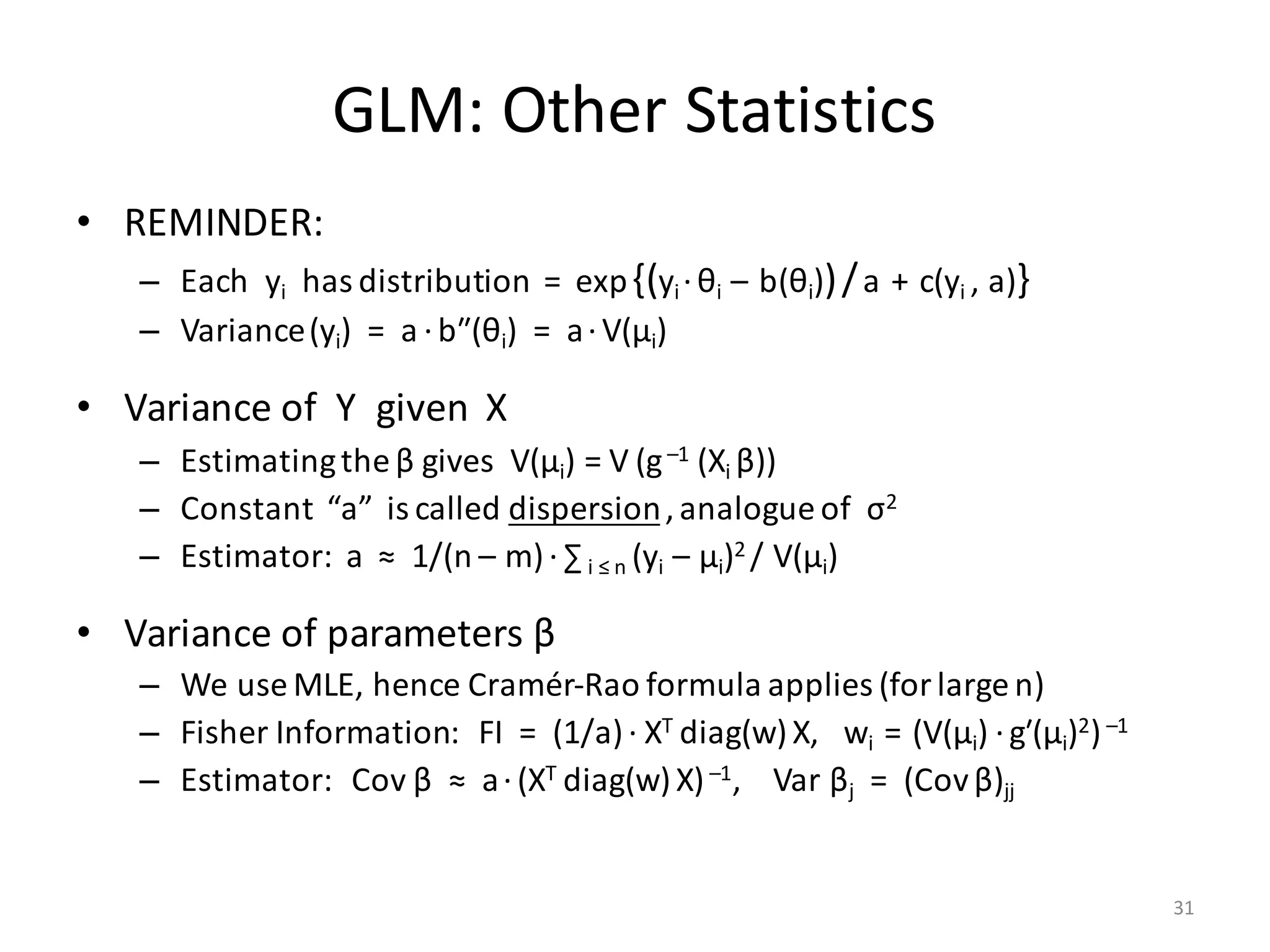
• GLM Regression:
– Each yi has distribution = exp{(yi ·θi – b(θi))/a + c(yi , a)}
– Canonical parameter θi represents the mean: μi = bʹ(θi)
– Link function connects μi and Xi β* : Xi β* = g(μi), μi = g –1 (Xi β*)
– Variance(yi) = a ·bʺ(θi)
• Why θi ? What is b(θi)?
– θi makes formulas simpler, stands for μi (no big deal)
– b(θi) defines what distribution it is: linear, logistic, Poisson, etc.
– b(θi) connects mean with variance: Var(yi) = a·bʺ(θi), μi = bʹ(θi)
• What is link function?
– You choose it to link μi with your features β1xi1 + β2xi2 + … + βmxim
– Additive effects: μi = Xi β; Multiplicative effects: μi = exp(Xi β)
Bayes law effects: μi = 1 / (1 + exp (– Xi β)); Inverse: μi = 1 / (Xi β)
– Xi β has range (– ∞, +∞), but μi may range in [0, 1], [0, +∞) etc.
22](https://image.slidesharecdn.com/s3regressionlesson-160913183002/75/Regression-using-Apache-SystemML-by-Alexandre-V-Evfimievski-22-2048.jpg)
![Trust Region Conj. Gradient
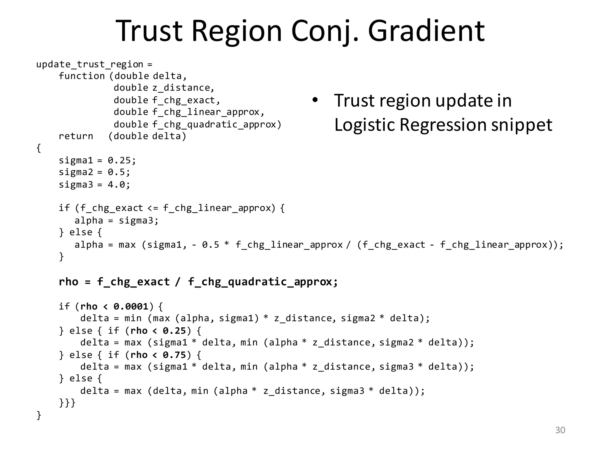
• Code snippet for
Logistic Regression
g = - 0.5 * t(X) %*% y; f_val = - N * log (0.5);
delta = 0.5 * sqrt (D) / max (sqrt (rowSums (X ^ 2)));
exit_g2 = sum (g ^ 2) * tolerance ^ 2;
while (sum (g ^ 2) > exit_g2 & i < max_i)
{
i = i + 1;
r = g;
r2 = sum (r ^ 2); exit_r2 = 0.01 * r2;
d = - r;
z = zeros_D; j = 0; trust_bound_reached = FALSE;
while (r2 > exit_r2 & (! trust_bound_reached) & j < max_j)
{
j = j + 1;
Hd = lambda * d + t(X) %*% diag (w) %*% X %*% d;
c = r2 / sum (d * Hd);
[c, trust_bound_reached] = ensure_quadratic (c, sum(d^2), 2 * sum(z*d), sum(z^2) - delta^2);
z = z + c * d;
r = r + c * Hd;
r2_new = sum (r ^ 2);
d = - r + (r2_new / r2) * d;
r2 = r2_new;
}
p = 1.0 / (1.0 + exp (- y * (X %*% (beta + z))));
f_chg = - sum (log (p)) + 0.5 * lambda * sum ((beta + z) ^ 2) - f_val;
delta = update_trust_region (delta, sqrt(sum(z^2)), f_chg, sum(z*g), 0.5 * sum(z*(r + g)));
if (f_chg < 0)
{
beta = beta + z;
f_val = f_val + f_chg;
w = p * (1 - p);
g = - t(X) %*% ((1 - p) * y) + lambda * beta;
} }
ensure_quadratic =
function (double x, a, b, c)
return (double x_new, boolean test)
{
test = (a * x^2 + b * x + c > 0);
if (test) {
rad = sqrt (b ^ 2 - 4 * a * c);
if (b >= 0) {
x_new = - (2 * c) / (b + rad);
} else {
x_new = - (b - rad) / (2 * a);
}
} else {
x_new = x;
} }
29](https://image.slidesharecdn.com/s3regressionlesson-160913183002/75/Regression-using-Apache-SystemML-by-Alexandre-V-Evfimievski-29-2048.jpg)
![GLM: Deviance
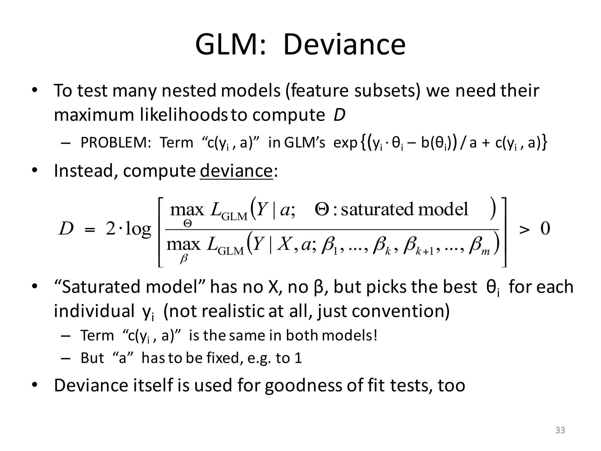
• Let X have m features, of which k may have no effect on Y
– Will “no effect” result in βj ≈ 0 ? (Unlikely.)
– Estimate βj and Var βj then test βj / (Var βj)1/2 against N(0, 1)?
• Student’s t-test is better
• Likelihood Ratio Test:
• Null Hypothesis: Y given X follows GLM with β1 = … = βk = 0
– If NH is true, D is asympt. distributed as χ2 with k deg. of freedom
– If NH is false, D → +¥as n → +¥
• P-value % = Prob[ χ2
k > D] · 100%
( )
( )
0
...,,,0...,,0;,|max
...,,,...,,;,|max
log2
1GLM
11GLM
>
⎥
⎥
⎦
⎤
⎢
⎢
⎣
⎡
⋅=
+
+
mk
mkk
aXYL
aXYL
D
ββ
ββββ
β
β
32](https://image.slidesharecdn.com/s3regressionlesson-160913183002/75/Regression-using-Apache-SystemML-by-Alexandre-V-Evfimievski-32-2048.jpg)
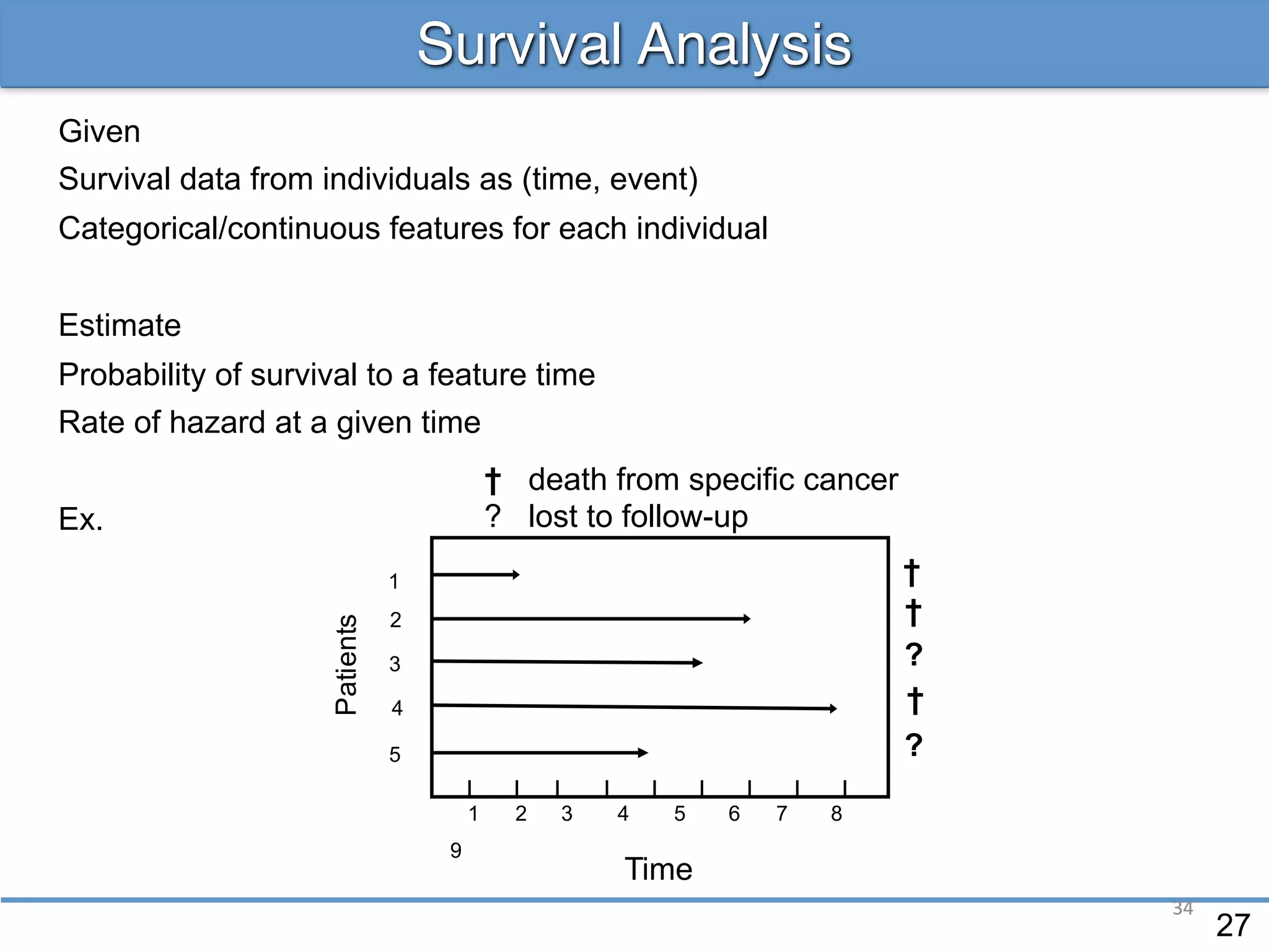
![36
Event Hazard Rate
• Symptom events E follow a Poisson process:
timeE1 E2 E3 E4
Death
Hazard
function
Hazard function = Poisson rate:
Given state and hazard, we could compute the probability of the
observed event count:
[ ]
t
tttE
th
t Δ
Δ+∈
=
→Δ
state),[Prob
limstate);(
|
0
[ ] ,
!
ineventsProb 21
K
He
tttK
KH−
=≤≤ dttthH
t
t
))(state;(
2
1
∫=](https://image.slidesharecdn.com/s3regressionlesson-160913183002/75/Regression-using-Apache-SystemML-by-Alexandre-V-Evfimievski-36-2048.jpg)
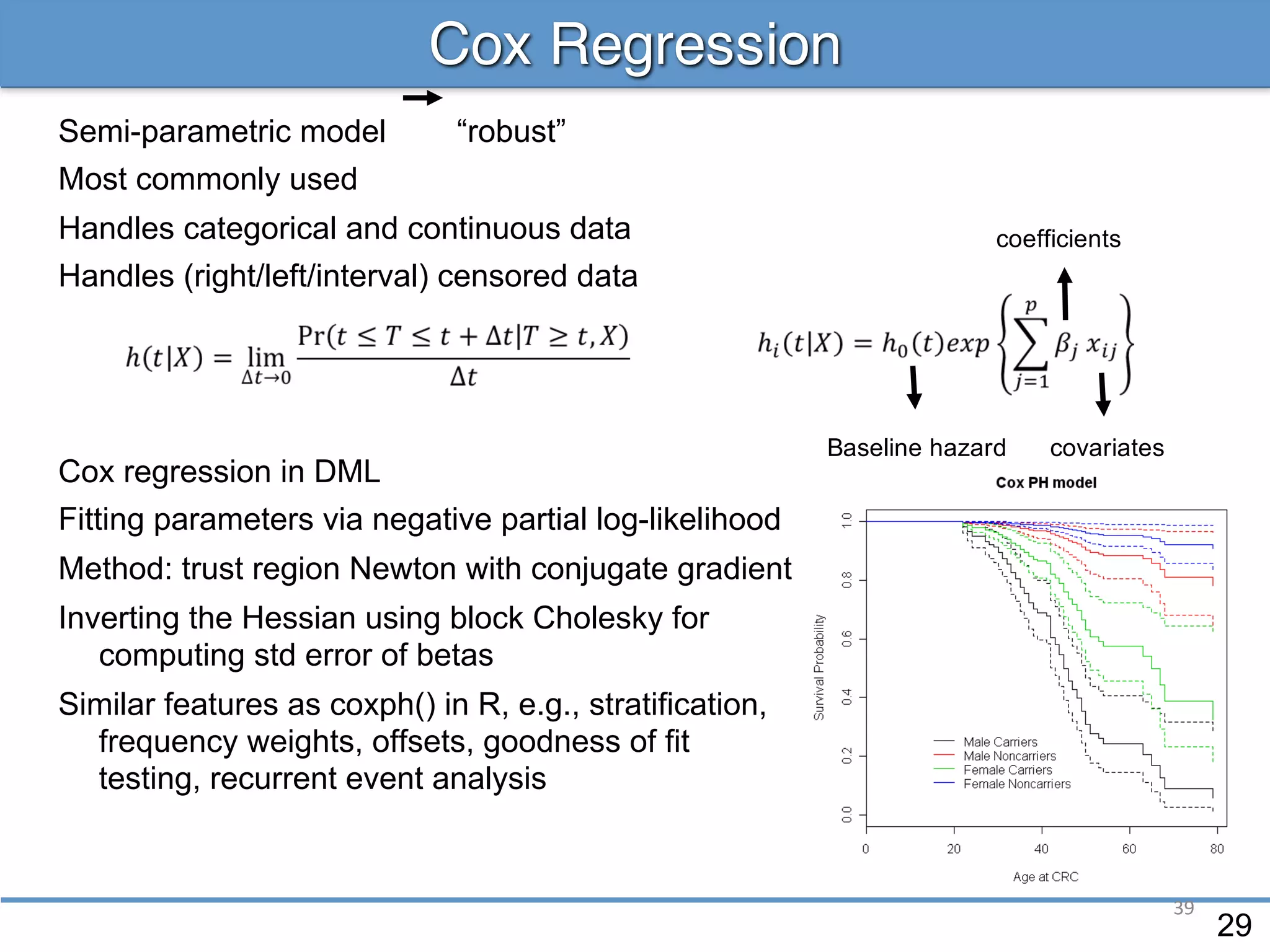
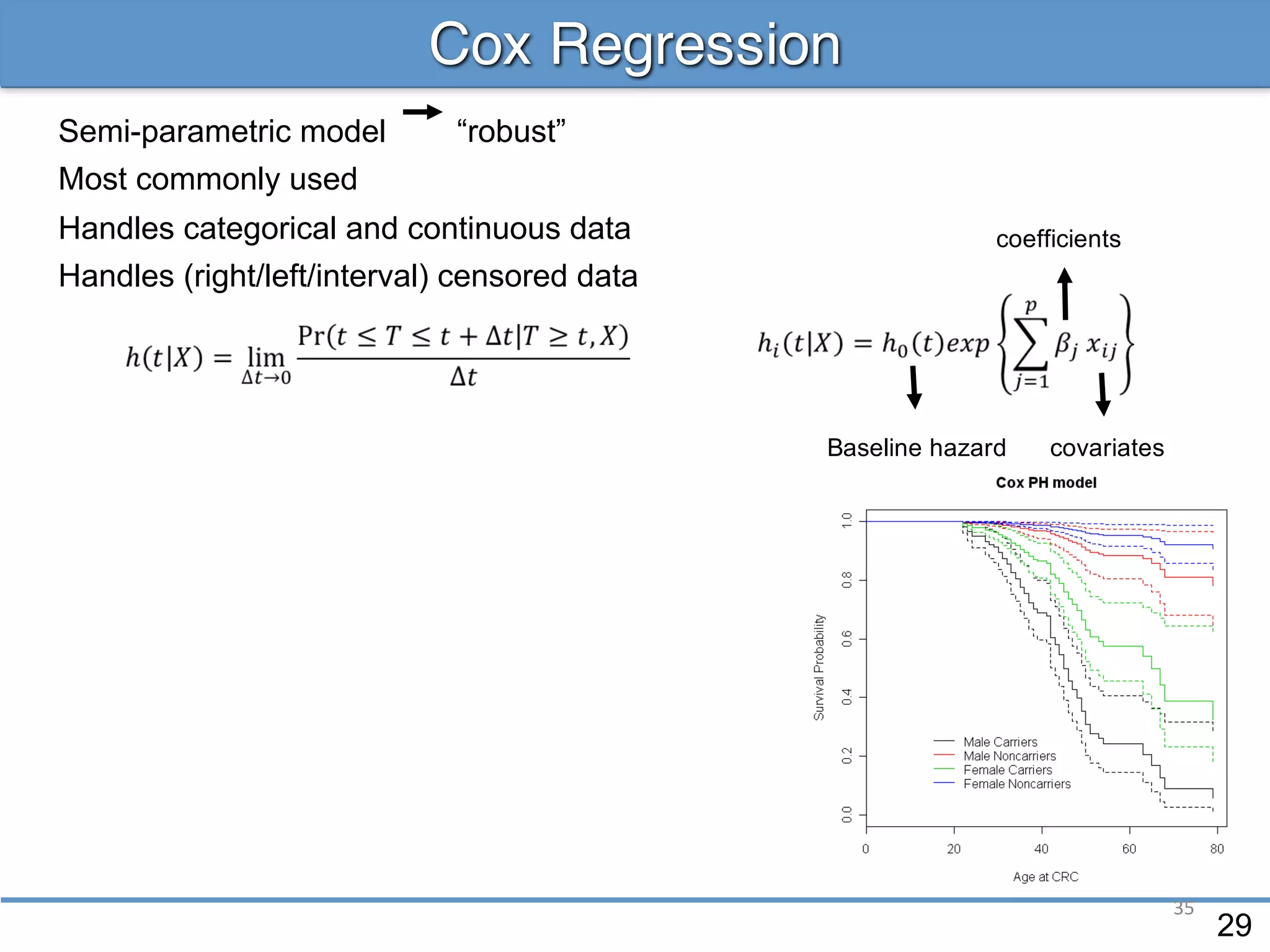
![37
Cox Proportional Hazards
• Assume that exactly 1 patient gets event E at time t
• The probability that it is Patient #i is the hazard ratio:
• Cox assumption:
• Time confounder cancels out!
t
[ ] ∑ =
=
n
j ji sthsthEi 1
);();(gets#Prob
s1
si = statei
s2
sn
Patient #1
Patient #2
Patient #3
Patient #n – 1
Patient #n
. . . . .
)(exp)((state))(state);( T
00 sththth λ⋅=Λ⋅=](https://image.slidesharecdn.com/s3regressionlesson-160913183002/75/Regression-using-Apache-SystemML-by-Alexandre-V-Evfimievski-37-2048.jpg)
![38
Cox “Partial” Likelihood
• Cox “partial” likelihood for the dataset is a product over all E:
Patient #1
Patient #2
Patient #3
Patient #n – 1
Patient #n
. . . . .
[ ] ∏
∑
∏
∑ ==
=== EtEt n
j j
t
n
j j
t
ts
ts
tsth
tsth
EL ::
1
T
)(who
T
1
)(who
Cox
)(
)(
)(
)(
)(exp
)(exp
)(;
)(;
allProb)(
λ
λ
λ](https://image.slidesharecdn.com/s3regressionlesson-160913183002/75/Regression-using-Apache-SystemML-by-Alexandre-V-Evfimievski-38-2048.jpg)