Downloaded 320 times


![Convex Optimization
Setting: G : H R ⇤ {+⇥}
H: Hilbert space. Here: H = RN .
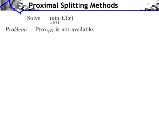
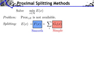
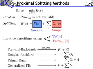
Problem: min G(x)
x H
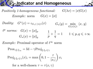
Class of functions: x y
Convex: G(tx + (1 t)y) tG(x) + (1 t)G(y) t [0, 1]](https://image.slidesharecdn.com/course-signal-convex-optimization-121213052433-phpapp02/85/Signal-Processing-Course-Convex-Optimization-3-320.jpg)
![Convex Optimization
Setting: G : H R ⇤ {+⇥}
H: Hilbert space. Here: H = RN .
Problem: min G(x)
x H
Class of functions: x y
Convex: G(tx + (1 t)y) tG(x) + (1 t)G(y) t [0, 1]
Lower semi-continuous: lim inf G(x) G(x0 )
x x0
Proper: {x ⇥ H G(x) ⇤= + } = ⌅
⇤](https://image.slidesharecdn.com/course-signal-convex-optimization-121213052433-phpapp02/85/Signal-Processing-Course-Convex-Optimization-4-320.jpg)
![Convex Optimization
Setting: G : H R ⇤ {+⇥}
H: Hilbert space. Here: H = RN .
Problem: min G(x)
x H
Class of functions: x y
Convex: G(tx + (1 t)y) tG(x) + (1 t)G(y) t [0, 1]
Lower semi-continuous: lim inf G(x) G(x0 )
x x0
Proper: {x ⇥ H G(x) ⇤= + } = ⌅
⇤
0 if x ⇥ C,
Indicator: C (x) =
+ otherwise.
(C closed and convex)](https://image.slidesharecdn.com/course-signal-convex-optimization-121213052433-phpapp02/85/Signal-Processing-Course-Convex-Optimization-5-320.jpg)
![Sub-differential
Sub-di erential:
G(x) = {u ⇥ H ⇤ z, G(z) G(x) + ⌅u, z x⇧}
G(x) = |x|
G(0) = [ 1, 1]](https://image.slidesharecdn.com/course-signal-convex-optimization-121213052433-phpapp02/85/Signal-Processing-Course-Convex-Optimization-11-320.jpg)
![Sub-differential
Sub-di erential:
G(x) = {u ⇥ H ⇤ z, G(z) G(x) + ⌅u, z x⇧}
G(x) = |x|
Smooth functions:
If F is C 1 , F (x) = { F (x)}
G(0) = [ 1, 1]](https://image.slidesharecdn.com/course-signal-convex-optimization-121213052433-phpapp02/85/Signal-Processing-Course-Convex-Optimization-12-320.jpg)
![Sub-differential
Sub-di erential:
G(x) = {u ⇥ H ⇤ z, G(z) G(x) + ⌅u, z x⇧}
G(x) = |x|
Smooth functions:
If F is C 1 , F (x) = { F (x)}
G(0) = [ 1, 1]
First-order conditions:
x argmin G(x) 0 G(x )
x H](https://image.slidesharecdn.com/course-signal-convex-optimization-121213052433-phpapp02/85/Signal-Processing-Course-Convex-Optimization-13-320.jpg)
![Sub-differential
Sub-di erential:
G(x) = {u ⇥ H ⇤ z, G(z) G(x) + ⌅u, z x⇧}
G(x) = |x|
Smooth functions:
If F is C 1 , F (x) = { F (x)}
G(0) = [ 1, 1]
First-order conditions:
x argmin G(x) 0 G(x )
x H U (x)
x
Monotone operator: U (x) = G(x)
(u, v) U (x) U (y), y x, v u 0](https://image.slidesharecdn.com/course-signal-convex-optimization-121213052433-phpapp02/85/Signal-Processing-Course-Convex-Optimization-14-320.jpg)
![1
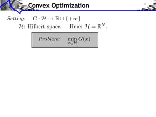
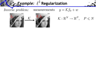
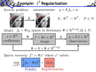
Example: Regularization
1
x ⇥ argmin G(x) = ||y x||2 + ||x||1
x RQ 2
⇥G(x) = ( x y) + ⇥|| · ||1 (x)
sign(xi ) if xi ⇥= 0,
|| · ||1 (x)i =
[ 1, 1] if xi = 0.](https://image.slidesharecdn.com/course-signal-convex-optimization-121213052433-phpapp02/85/Signal-Processing-Course-Convex-Optimization-15-320.jpg)
![1
Example: Regularization
1
x ⇥ argmin G(x) = ||y x||2 + ||x||1
x RQ 2
⇥G(x) = ( x y) + ⇥|| · ||1 (x)
sign(xi ) if xi ⇥= 0, xi
|| · ||1 (x)i =
[ 1, 1] if xi = 0.
i
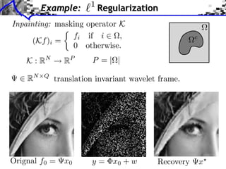
Support of the solution:
I = {i ⇥ {0, . . . , N 1} xi ⇤= 0}](https://image.slidesharecdn.com/course-signal-convex-optimization-121213052433-phpapp02/85/Signal-Processing-Course-Convex-Optimization-16-320.jpg)
![1
Example: Regularization
1
x ⇥ argmin G(x) = ||y x||2 + ||x||1
x RQ 2
⇥G(x) = ( x y) + ⇥|| · ||1 (x)
sign(xi ) if xi ⇥= 0, xi
|| · ||1 (x)i =
[ 1, 1] if xi = 0.
i
Support of the solution:
I = {i ⇥ {0, . . . , N 1} xi ⇤= 0}
First-order conditions: i, y x
i
s RN , ( x y) + s = 0
sI = sign(xI ),
||sI c || 1.](https://image.slidesharecdn.com/course-signal-convex-optimization-121213052433-phpapp02/85/Signal-Processing-Course-Convex-Optimization-17-320.jpg)
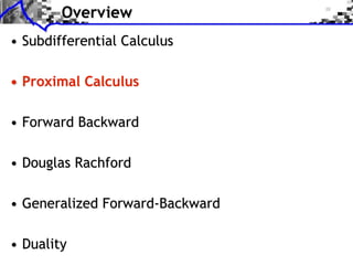
![Gradient and Proximal Descents
Gradient descent: x( +1) = x( ) G(x( ) ) [explicit]
G is C 1 and G is L-Lipschitz
Theorem: If 0 < < 2/L, x( )
x a solution.](https://image.slidesharecdn.com/course-signal-convex-optimization-121213052433-phpapp02/85/Signal-Processing-Course-Convex-Optimization-31-320.jpg)
![Gradient and Proximal Descents
Gradient descent: x( +1) = x( ) G(x( ) ) [explicit]
G is C 1 and G is L-Lipschitz
Theorem: If 0 < < 2/L, x( )
x a solution.
Sub-gradient descent: x( +1)
= x( )
v( ) , v( )
G(x( ) )
Theorem: If 1/⇥, x( )
x a solution.
Problem: slow.](https://image.slidesharecdn.com/course-signal-convex-optimization-121213052433-phpapp02/85/Signal-Processing-Course-Convex-Optimization-32-320.jpg)
![Gradient and Proximal Descents
Gradient descent: x( +1) = x( ) G(x( ) ) [explicit]
G is C 1 and G is L-Lipschitz
Theorem: If 0 < < 2/L, x( )
x a solution.
Sub-gradient descent: x( +1)
= x( )
v( ) , v( )
G(x( ) )
Theorem: If 1/⇥, x( )
x a solution.
Problem: slow.
Proximal-point algorithm: x(⇥+1) = Prox G (x(⇥) ) [implicit]
Theorem: If c > 0, x( )
x a solution.
Prox G hard to compute.](https://image.slidesharecdn.com/course-signal-convex-optimization-121213052433-phpapp02/85/Signal-Processing-Course-Convex-Optimization-33-320.jpg)

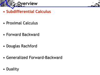
![Block Regularization
1 2
block sparsity: G(x) = ||x[b] ||, ||x[b] ||2 = x2
m
b B m b
iments Towards More Complex Penalization
(2) Bk
2
+ ` 1 `2
4
k=1 x 1,2
b B1 i b xi
⇥ x⇥⇥1 = i ⇥xi ⇥ b B i b xi2 +
i b xi
N: 256
b B2
b B
Image f = x Coe cients x.](https://image.slidesharecdn.com/course-signal-convex-optimization-121213052433-phpapp02/85/Signal-Processing-Course-Convex-Optimization-68-320.jpg)
![Block Regularization
1 2
block sparsity: G(x) = ||x[b] ||, ||x[b] ||2 = x2
m
b B m b
iments Towards More Complex Penalization
Non-overlapping decomposition: B = B ... B
Towards More Complex Penalization
Towards More Complex Penalization
n
1 n
2 G(x) =4 x iBk
(2)
+ ` ` k=1 G 1,2
(x) Gi (x) = ||x[b] ||,
1 2 i=1 b Bi
b b 1b1 B1 i b xiixb xi
22
BB
⇥ x⇥x⇥x⇥⇥1 =i ⇥x⇥x⇥xi ⇥
⇥= ++ +
i b i
⇥ ⇥1 ⇥1 = i i ⇥i i ⇥ bb B B i
Bb xii2bi2xi2
bbx
i
N: 256
b b 2b2 B2 i
BB xi2 b2xi
b b xi
i
b B
Image f = x Coe cients x. Blocks B1 B1 B2](https://image.slidesharecdn.com/course-signal-convex-optimization-121213052433-phpapp02/85/Signal-Processing-Course-Convex-Optimization-69-320.jpg)
![Block Regularization
1 2
block sparsity: G(x) = ||x[b] ||, ||x[b] ||2 = x2
m
b B m b
iments Towards More Complex Penalization
Non-overlapping decomposition: B = B ... B
Towards More Complex Penalization
Towards More Complex Penalization
n
1 n
2 G(x) =4 x iBk
(2)
+ ` ` k=1 G 1,2
(x) Gi (x) = ||x[b] ||,
1 2 i=1 b Bi
Each Gi is simple: b b 1b1 B1 i b xiixb xi
BB
22
⇥ x⇥x⇥x⇥⇥1 =i ⇥xG ⇥xi ⇥ m = b B B i b xii2bi2xi2
⇥ ⇥1 = i ⇥i i x +
i b i
⇤ m ⇥ b ⇥ Bi , ⇥ ⇥1Prox i ⇥xi ⇥(x) b max i0, 1
= Bb bx ++m
N: 256 ||x[b]b||B xi2 b2xi
2 2 B2
b B b i b b xi
i
b B
Image f = x Coe cients x. Blocks B1 B1 B2](https://image.slidesharecdn.com/course-signal-convex-optimization-121213052433-phpapp02/85/Signal-Processing-Course-Convex-Optimization-70-320.jpg)
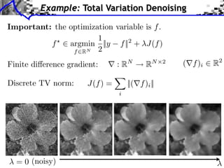
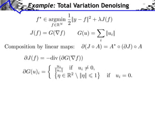
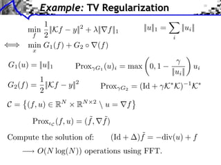
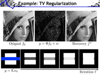
![Example: TV Denoising
1
min ||f y||2 + ||⇥f ||1 min ||y + div(u)||2
f RN 2 ||u||
||u||1 = ||ui || ||u|| = max ||ui ||
i
i
Dual solution u Primal solution f = y + div(u )
[Chambolle 2004]](https://image.slidesharecdn.com/course-signal-convex-optimization-121213052433-phpapp02/85/Signal-Processing-Course-Convex-Optimization-86-320.jpg)
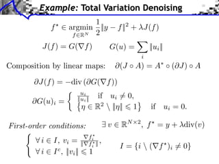
![Example: TV Denoising
1
min ||f y||2 + ||⇥f ||1 min ||y + div(u)||2
f RN 2 ||u||
||u||1 = ||ui || ||u|| = max ||ui ||
i
i
Dual solution u Primal solution f = y + div(u )
FB (aka projected gradient descent): [Chambolle 2004]
u( +1)
= Proj||·|| u( ) + (y + div(u( ) ))
ui
v = Proj||·|| (u) vi =
max(||ui ||/ , 1)
2 1
Convergence if < =
||div ⇥|| 4](https://image.slidesharecdn.com/course-signal-convex-optimization-121213052433-phpapp02/85/Signal-Processing-Course-Convex-Optimization-87-320.jpg)
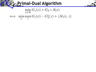
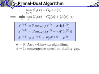
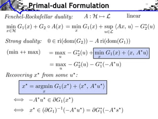
![Primal-Dual Algorithm
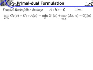
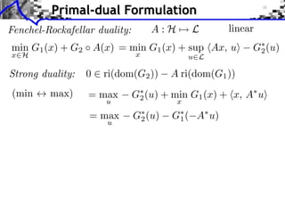
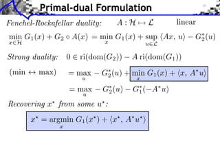
min G1 (x) + G2 A(x)
x H
() min max G1 (x) G⇤ (z) + hA(x), zi
2
x z
z (`+1) = Prox G⇤
2
(z (`) + A(˜(`) )
x
x(⇥+1) = Prox G1 (x(⇥) A (z (⇥) ))
˜
x( +1)
= x( +1)
+ (x( +1)
x( ) )
= 0: Arrow-Hurwicz algorithm.
= 1: convergence speed on duality gap.
Theorem: [Chambolle-Pock 2011]
If 0 1 and ⇥⇤ ||A||2 < 1 then
x( )
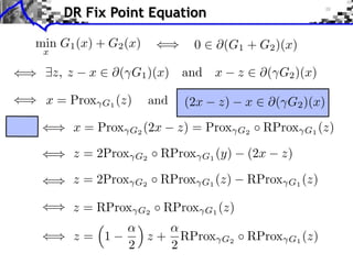
x minimizer of G1 + G2 A.](https://image.slidesharecdn.com/course-signal-convex-optimization-121213052433-phpapp02/85/Signal-Processing-Course-Convex-Optimization-90-320.jpg)

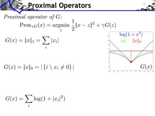
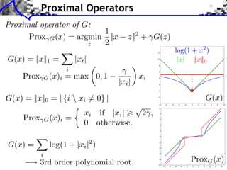
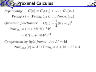
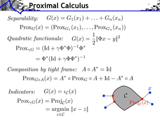
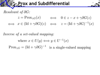
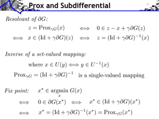
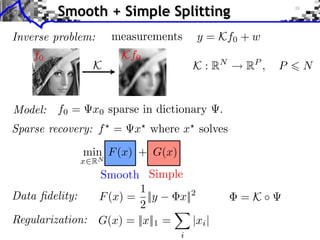
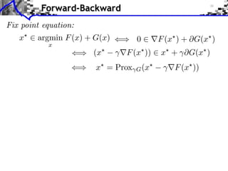
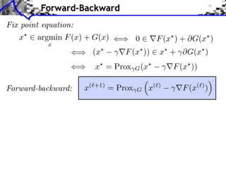
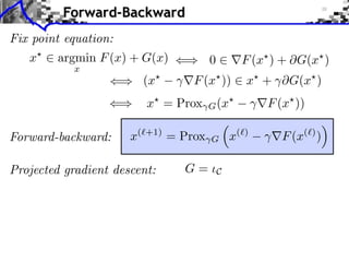
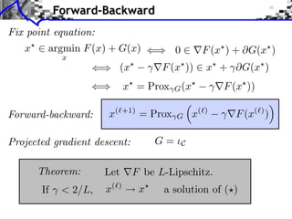
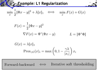
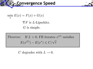
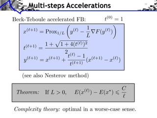
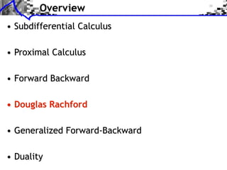
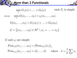
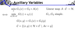
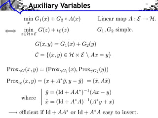
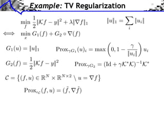
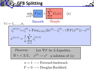
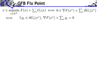
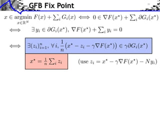
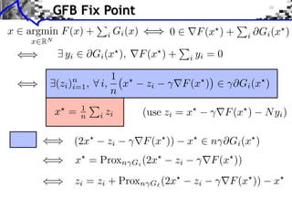
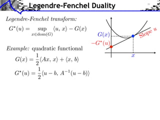
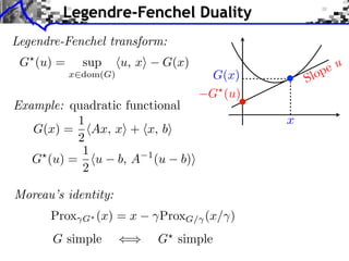
This document discusses convex optimization and proximal operators. It begins by introducing convex optimization problems with objective functions G mapping from a Hilbert space H to the real numbers. It then discusses properties of convex, lower semi-continuous, and proper functions. Examples are given of regularization problems and total variation denoising. The document covers subdifferentials, proximal operators, proximal calculus including separability and compositions, and relationships between proximal operators and subdifferentials. Gradient descent and subgradient descent algorithms are also briefly discussed.