Fitting a model to data is typically done by finding the parameter values that minimize some loss function.
There are many possible loss functions. What criterion should we use for choosing one?
Choose one that makes the math easy (squared error)
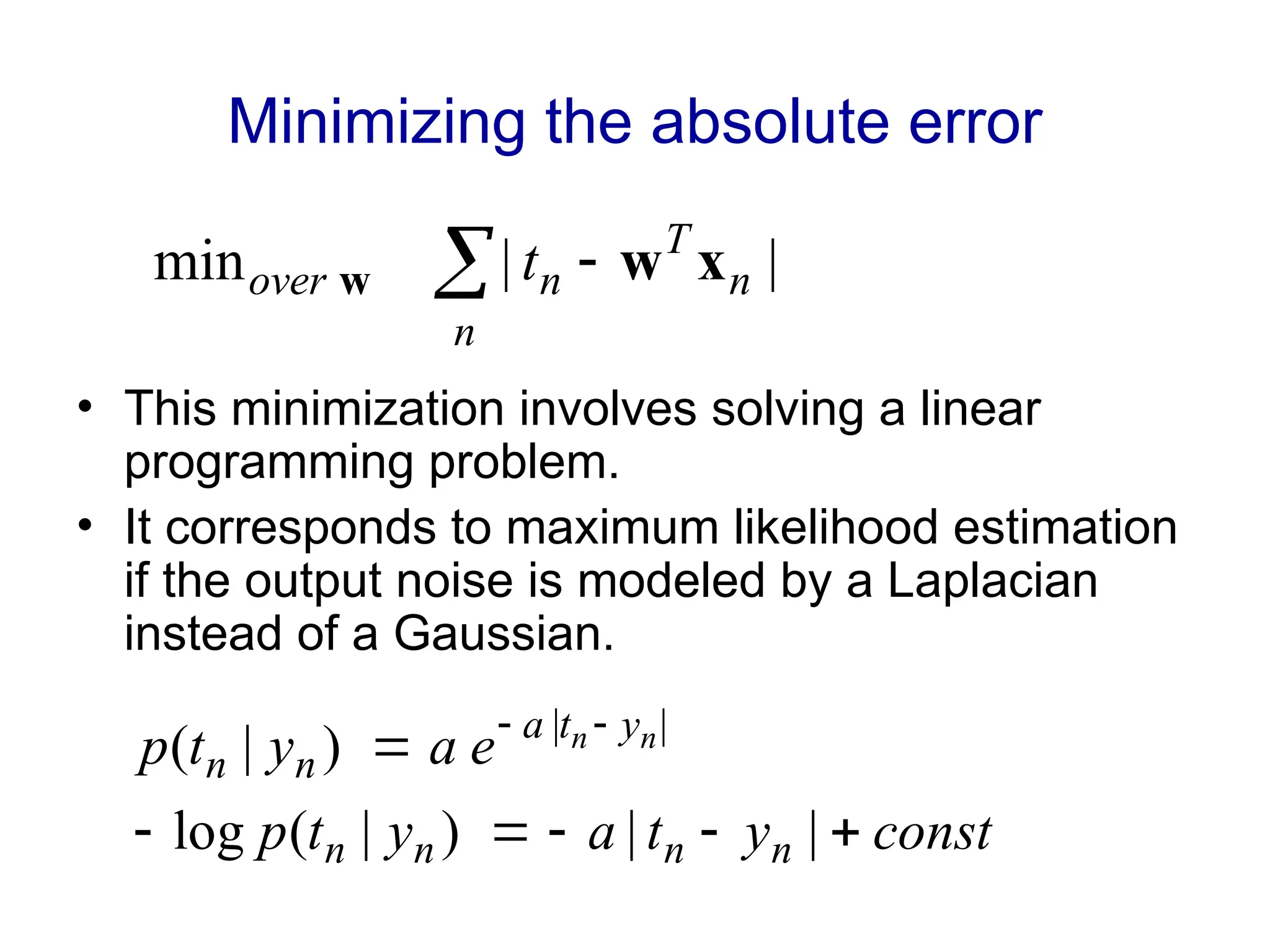
Choose one that makes the fitting correspond to maximizing the likelihood of the training data given some noise model for the observed outputs.
Choose one that makes it easy to interpret the learned coefficients (easy if mostly zeros)
Choose one that corresponds to the real loss on a practical application (losses are often asymmetric)