The document outlines the processes involved in data preparation, including pre-processing and descriptive statistics using SystemML. It covers various aspects such as the transformation of input data, training and testing data sets, and detailed statistical measures for analyzing data relationships. The procedures and built-in functions for handling categorical variables, cross-validation methods, and criteria for descriptive statistics are also discussed.

1. Data Preparation and
Descriptive Statistics in
SystemML
1

2. Outline
• Data pre-processing and transformation
• Training/Testing/Cross Validation
• Descriptive statistics
I. Univariate statistics
II. Bivariate statistics
III. Stratified statistics
2

3. Input Data Format
3
Input data
§ Rows: data points (aka records)
§ Columns: features (aka variables, attributes)
Feature types:
§ Scale (aka continuous), e.g., ‘Height’, ‘Weight’, ‘Salary’, ‘Temperature’
§ Categorical (aka discrete)
§ Nominal – no natural ranking, e.g., ‘Gender’, ‘Region’, ‘Hair color’
§ Ordinal – natural ranking, e.g., ‘Level of Satisfaction’
Example:
The house data set

4. Data Pre-Processing
Tabular input data needs to be transformed into a matrix – transform() built-in function
Categorical features need special treatment:
§ Recoding: mapping distinct categories into consecutive numbers starting from 1
§ Dummycoding (aka one-hot-encoding, one-of-K encoding)
Example:
recoding dummycoding
4
Zipcode
96334
95123
95141
96334
Zipcode
1
2
3
1
direction
east
west
north
south
dir_east dir_west dir_north dir_south
1 0 0 0
0 1 0 0
0 0 1 0
0 0 0 1

5. transform() Built-in Function
transform() built-in function supports:
§ Omitting missing values
§ Missing value imputation by global_mean (scale features), global_mode (categorical
features), or constant (scale/categorical features)
§ Binning (equi-width)
§ Scaling (scale features): mean-subtraction, z-score
§ Recoding
§ Dummycoding
5

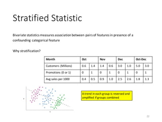
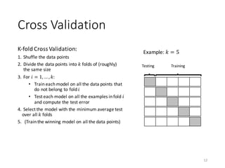
6. Transform Specification
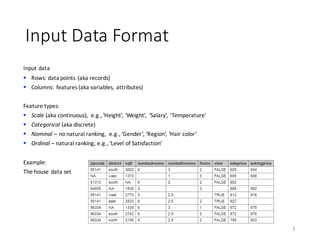
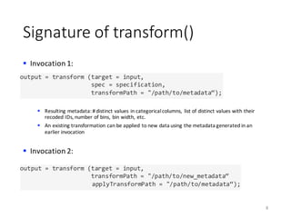
§ Transformations operate on individual columns
§ All required transformations specified in a JSON file
§ Property na.strings in the mtd file specifies missing values
Example:
data.spec.json data.csv.mtd
6
{
"data_type": "frame",
"format": "csv",
"sep": ",",
"header": true,
"na.strings": [ "NA", "" ]
}
{
“ids": true
, "omit": [ 1, 4, 5, 6, 7, 8, 9 ]
, "impute":
[ { “id": 2, "method": "constant",
"value": "south" }
,{ “id": 3, "method":
"global_mean" }
]
,"recode": [ 1, 2, 4, 5, 6, 7 ]
,"bin":
[ { “id": 8, "method": "equi-
width", "numbins": 3 } ]
,"dummycode": [ 2, 5, 6, 7, 8, 3 ]
}

7. Combinations of Transformations
7

8. Signature of transform()
§ Invocation 1:
§ Resulting metadata: # distinct values in categorical columns, list of distinct values with their
recoded IDs, number of bins, bin width, etc.
§ An existing transformation can be applied to new data using the metadata generated in an
earlier invocation
§ Invocation 2:
8
output = transform (target = input,
spec = specification,
transformPath = "/path/to/metadata“);
output = transform (target = input,
transformPath = "/path/to/new_metadata“
applyTransformPath = "/path/to/metadata“);

9. Outline
• Data pre-processing and transformation
• Training/Testing/Cross Validation
• Descriptive statistics
I. Univariate statistics
II. Bivariate statistics
III. Stratified statistics
9

10. Training/Testing
§ Pre-processing training and testing data sets
§ Splitting data points and labels – splitXY.dml and splitXY-dummy.dml (hands-on)
§ Sampling data points – sample.dml (hands-on)
§ Cross Validation – cv-linreg.dml (hands-on)
10

11. Pre-Processing Training and
Testing Data
Training phase
Testing phase
11
Train = read ("/user/ml/trainset.csv");
Spec = read("/user/ml/tf.spec.json“, data_type = "scalar",
value_type = "String");
trainD = transform (target = Train,
transformSpec = Spec,
transformPath = "/user/ml/train_tf_metadata");
# Build a predictive model using trainD
...
Test = read ("/user/ml/testset.csv");
testD = transform (target = Test,
transformPath = "/user/ml/test_tf_metadata",
applyTransformPath = "/user/ml/train_tf_metdata");
# Test the model using testD
...

12. Cross Validation
K-fold Cross Validation:
1. Shuffle the data points
2. Divide the data points into 𝑘 folds of (roughly)
the same size
3. For 𝑖 = 1, … , 𝑘:
• Train each model on all the data points that
do not belong to fold 𝑖
• Test each model on all the examples in fold 𝑖
and compute the test error
4. Select the model with the minimum average test
over all 𝑘 folds
5. (Train the winning model on all the data points)
12
Testing Training
Example: 𝑘 = 5

13. Outline
• Data pre-processing and transformation
• Training/Testing/Cross Validation
• Descriptive statistics
I. Univariate statistics
II. Bivariate statistics
III. Stratified statistics
13

14. Univariate Statistics
14
Row Name of Statistic Scale Category
1 Minimum +
2 Maximum +
3 Range +
4 Mean +
5 Variance +
6 Standard deviation +
7 Standard error of mean +
8 Coefficient of variation +
9 Skewness +
10 Kurtosis +
11 Standard error of skewness +
12 Standard error of Kurtosis +
13 Median +
14 Intequartilemean +
15 Number of categories +
16 Mode +
17 Number of modes +
Central tendency measures
Dispersion measures
Shape measures
Categorical measures

15. Bivariate Statistics
Quantitative association between pairs of features
I. Scale-vs-Scale statistics
§ Pearson’s correlation coefficient
II. Nominal-vs-Nominal statistics
§ Pearson’s 𝜒)
§ Cramér's 𝑉
III. Nominal-vs-Scale statistics
§ Eta statistic
§ 𝐹 statistic
IV. Ordinal-vs-Ordinal statistics
§ Spearman’s rank correlation coefficient
15

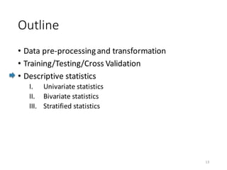
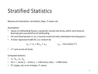
16. Scale-vs-Scale Statistics
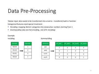
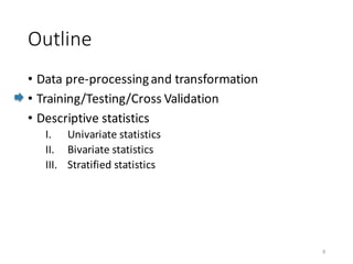
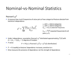
Pearson’s correlation coefficient
§ A measure of linear dependence between scale features
§ 𝜌)
measures accuracy of 𝑥) ~ 𝑥0
16
𝜌 =
123(56,57)
9:69:7
, 𝜌 ∈ [−1,+1]
1 − 𝜌)
=
∑ 𝑥A,) − 𝑥BA,)
)C
AD0
∑ 𝑥A,) − 𝑥̅A,)
)C
AD0
Residual Sum of Squares (RSS)
Total Sum of Squares (TSS)

17. Nominal-vs-Nominal Statistics
Pearson’s 𝜒)
§ A measure how much frequencies of value pairs of two categorical features deviate from
statistical independence
§ Under independence assumption Pearson’s 𝜒)
distributed approximately 𝜒)
𝑑 with
𝑑 = (𝑘0 − 1)(𝑘) − 1) degrees of freedom
§ 𝑃-value:
§ 𝑃 → 0 (rapidly) as features’ dependence increases, sensitive to 𝑛
§ Only measures the presence of dependence not the strength of dependence
17
𝜒)
= K
𝑂M,N − 𝐸M,N
)
𝐸M,NM,N
𝑥0 with 𝑘0 distinct categories
𝑥) with 𝑘) distinct categories
𝑂M ,N = #(𝑎, 𝑏) observed frequencies
𝐸M,N =
#M #N
C
expected frequencies for all
pairs (𝑎, 𝑏)
𝑃 = Pr 𝜌 ≥ Pearson[
s 𝜒)
𝜌 ~𝜒)
(𝑑) distribution

18. Nominal-vs-Nominal Statistics
Cramér's 𝑉
§ A measure for the strength of association between two categorical features
§ Under independence assumption 𝑉 distributed approximately 𝜒)
𝑑 with
𝑑 = (𝑘0 − 1)(𝑘) − 1) degrees of freedom
§ 𝑃-value:
§ 𝑃 → 1 (slowly) as features’ dependence increases, sensitive to 𝑛
18
𝑉 =
Pearson[s 𝜒)
𝜒aM5
)
𝜒aM5
)
= 𝑛.min { 𝑘0 − 1, 𝑘) − 1}
𝑃 = Pr 𝜌 ≥ Cramér[
s 𝑉 𝜌 ~𝜒)
(𝑑) distribution

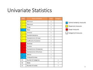
19. Nominal-vs-Scale Statistics
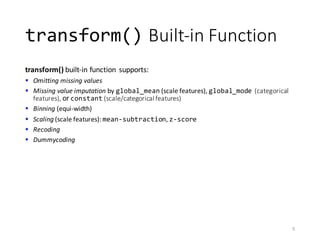
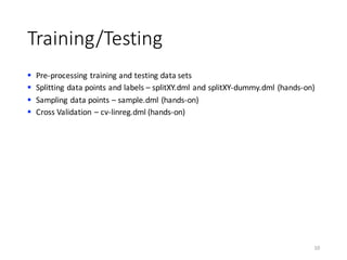
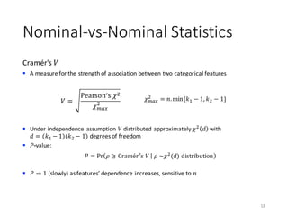
Eta statistic
§ A measure for the strength of association between a categorical feature and a scale
feature
§ 𝜂)
measures accuracy of 𝑦 ~ 𝑥 similar to 𝑅)
statistic of linear regression
19
𝜂)
= 1 −
∑ 𝑦A − 𝑦B[𝑥A] )C
AD0
∑ 𝑦A − 𝑦k )C
AD0
RSS
TSS
𝑥 categorical
𝑦 scale
𝑦B[𝑥A]: average of 𝑦A among all records with
𝑥A = 𝑥

20. Nominal-vs-Scale Statistics
𝐹 statistic
§ A measure for the strength of association between a categorical feature and a scale
feature
§ Assumptions (𝑥 categorical, 𝑦 scale):
§ 𝑦 ~ 𝑁𝑜𝑟𝑚𝑎𝑙 𝜇, 𝜎)
- same variance for all 𝑥
§ 𝑥 has small value domain with large frequency counts, 𝑥A non-random
§ All records are iid
§ Under independence assumption 𝐹 distributed approximately 𝐹(𝑘 − 1, 𝑛 − 𝑘)
20
𝐹 =
∑ 𝑓𝑟𝑒𝑞 𝑥 𝑦B 𝑥 − 𝑦k )/(𝑘 − 1)5
∑ 𝑦A − 𝑦B 𝑥A
)/(𝑛 − 𝑘)C
AD0
=
𝜂)(𝑛 − 𝑘)
1 − 𝜂)(𝑘 − 1)
ESS: Explained Sum of Squares
RSS
Degrees of freedom
Degrees of freedom

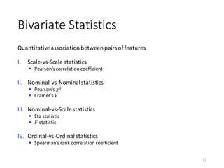
21. Ordinal-vs-Ordinal Statistics
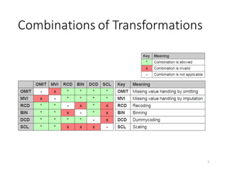
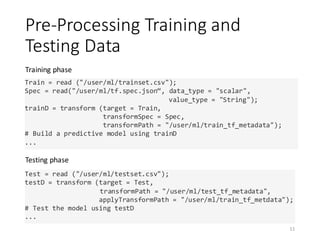
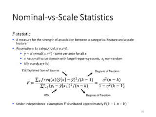
Spearman’s rank correlation coefficient
§ A measure for the strength of association between two ordinal features
§ Pearson’s correlation efficient applied to feature with values replaced by their ranks
Example:
21
8x
3)
11z
8{
5|
20
𝑥′
8
3
11
8
5
2
𝑥
4.5
2
6
4.5
3
1
𝑟
𝜌 =
123 (•6,•7)
9‚69‚7
𝜌 ∈ [−1, +1]

22. Stratified Statistic
Bivariate statistics measures association between pairs of features in presence of a
confounding categorical feature
Why stratification?
22
Month Oct Nov Dec Oct-Dec
Customers (Millions) 0.6 1.4 1.4 0.6 3.0 1.0 5.0 3.0
Promotions (0 or 1) 0 1 0 1 0 1 0 1
Avg sales per 1000 0.4 0.5 0.9 1.0 2.5 2.6 1.8 1.3
A trend in each group is reversed and
amplified if groups combined

23. Stratified Statistics
Measure of associations: correlation, slope, 𝑃-values, etc.
Assumptions:
• Values of confounding feature 𝑠 group the records into strata, within each strata all
bivariate pairs assumed free of confounding
• For each bivariate pair (𝑥, 𝑦), 𝑦 must be numerical and 𝑦 distributed normally given 𝑥
• A linear regression model for 𝑦 (𝑖: stratum id)
• 𝜎)
same across all strata
Computed statistics:
• 𝑥̅A, 𝜎„5…
, 𝑦kA, 𝜎B†…
• For 𝑥 ~ strata, y ~ strata, y ~ 𝑥 NO strata, and y ~ 𝑥 AND strata
• 𝑅)
, slopes, std. error of slopes, 𝑃- values
23
𝑦A,ˆ = 𝛼A + 𝛽𝑥A,ˆ + 𝜀A,ˆ 𝜀A,ˆ ~ 𝑁𝑜𝑟𝑚𝑎𝑙(0, 𝜎)
)