Download as PDF, PPTX


![Summarize all elements sik into the p × p sample variance-covariance matrix
S = sik i,k
.
Assume further, that the p × p population correlation matrix ρ is estimated by
the sample correlation matrix R with entries
rik =
sik
√
siiskk
, i = 1, . . . , p , k = 1, . . . , p ,
where rii = 1 for all i = 1, . . . , p.
> aimu <- read.table("aimu.dat", header=TRUE)
> attach(aimu)
> options(digits=2)
> mean(aimu[ ,3:8])
age height weight fvc fev1 fevp
30 177 77 553 460 83
4](https://image.slidesharecdn.com/multivriada-pptms-191117115606/85/Multivriada-ppt-ms-4-320.jpg)
![> cov(aimu[ ,3:8])
age height weight fvc fev1 fevp
age 110 -16.9 16.5 -233 -302 -20.8
height -17 45.5 34.9 351 275 -1.9
weight 16 34.9 109.6 325 212 -7.6
fvc -233 351.5 324.7 5817 4192 -86.5
fev1 -302 275.2 212.0 4192 4347 162.5
fevp -21 -1.9 -7.6 -87 162 41.3
> cor(aimu[ ,3:8])
age height weight fvc fev1 fevp
age 1.00 -0.239 0.15 -0.29 -0.44 -0.309
height -0.24 1.000 0.49 0.68 0.62 -0.043
weight 0.15 0.494 1.00 0.41 0.31 -0.113
fvc -0.29 0.683 0.41 1.00 0.83 -0.177
fev1 -0.44 0.619 0.31 0.83 1.00 0.384
fevp -0.31 -0.043 -0.11 -0.18 0.38 1.000
5](https://image.slidesharecdn.com/multivriada-pptms-191117115606/85/Multivriada-ppt-ms-5-320.jpg)

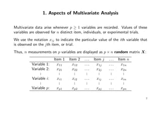
![Statistical distance should account for differences in variation and correlation.
Suppose we have n pairs of measurements on 2 independent variables x1 and x2:
> X <- mvrnorm(30, mu=c(0, 0), Sigma=matrix(c(9,0,0,1), 2, 2)); plot(X)
−6 −4 −2 0 2 4 6
−6−4−20246
X[,1]
X[,2]
Variability in x1 direction is much larger
than in x2 direction! Values that are a
given deviation from the origin in the
x1 direction are not as surprising as
are values in x2 direction.
It seems reasonable to weight an x2
coordinate more heavily than an x1
coordinate of the same value when
computing the distance to the origin.
7](https://image.slidesharecdn.com/multivriada-pptms-191117115606/85/Multivriada-ppt-ms-7-320.jpg)


![Example: Suppose x = (x1, x2)t
∼ N2(µ, Σ), with µ = (0, 0)t
and
Σ =
σ11 = 9 σ12 = 9/4
σ21 = 9/4 σ22 = 1
giving ρ12 = (9/4)/
√
9 · 1 = 3/4.
The eigen-analysis of Σ results in
> sigma <- matrix(c(9, 9/4, 9/4, 1), 2, 2)
> e <- eigen(sigma, symmetric=TRUE); e
$values
[1] 9.58939 0.41061
$vectors
[,1] [,2]
[1,] -0.96736 0.25340
[2,] -0.25340 -0.96736
19](https://image.slidesharecdn.com/multivriada-pptms-191117115606/85/Multivriada-ppt-ms-19-320.jpg)
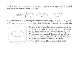
![−3 −2 −1 0 1 2 3
−3−2−10123
x1
x2 # check length of eigenvectors
> e$vectors[2,1]^2+e$vectors[1,1]^2
[1] 1
> e$vectors[2,2]^2+e$vectors[1,2]^2
[1] 1
# slopes of major & minor axes
> e$vectors[2,1]/e$vectors[1,1]
[1] 0.2619511
> e$vectors[2,2]/e$vectors[1,2]
[1] -3.817507
# endpoints of of major&minor axes
> sqrt(e$values[1])*e$vectors[,1]
[1] -2.9956024 -0.7847013
> sqrt(e$values[2])*e$vectors[,2]
[1] 0.1623767 -0.6198741
20](https://image.slidesharecdn.com/multivriada-pptms-191117115606/85/Multivriada-ppt-ms-20-320.jpg)


![Example cont’ed: Let again x = (x1, x2)t
∼ N2(µ, Σ), with µ = (0, 0)t
and
Σ =
9 9/4
9/4 1
=⇒ ρ =
1 3/4
3/4 1
.
The eigen-analysis of ρ now results in:
> rho <- matrix(c(1, 3/4, 3/4, 1), 2, 2)
> e <- eigen(rho, symmetric=TRUE); e
$values
[1] 1.75 0.25
$vectors
[,1] [,2]
[1,] 0.70711 0.70711
[2,] 0.70711 -0.70711
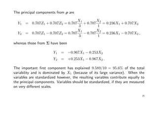
The total population variance is p = 2, and 1.75/2 = 87.5% of this variance is
already explained by the first principal component.
24](https://image.slidesharecdn.com/multivriada-pptms-191117115606/85/Multivriada-ppt-ms-24-320.jpg)
![Summarizing Sample Variation by Principal Components
So far we have dealt with population means µ and variances Σ. If we analyze a
sample then we have to replace Σ and µ by their empirical versions S and x.
The eigenvalues and eigenvectors are then based on S or R instead of Σ or ρ.
> library(mva)
> attach(aimu)
> options(digits=2)
> pca <- princomp(aimu[ , 3:8])
> summary(pca)
Importance of components:
Comp.1 Comp.2 Comp.3 Comp.4 Comp.5 Comp.6
Standard deviation 96.3 29.443 10.707 7.9581 4.4149 1.30332
Proportion of Variance 0.9 0.084 0.011 0.0061 0.0019 0.00016
Cumulative Proportion 0.9 0.981 0.992 0.9980 0.9998 1.00000
> pca$center # the means that were subtracted
age height weight fvc fev1 fevp
30 177 77 553 460 83
26](https://image.slidesharecdn.com/multivriada-pptms-191117115606/85/Multivriada-ppt-ms-26-320.jpg)
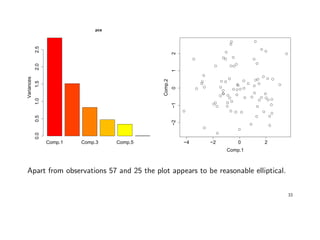
![> pca$scores # values of the p principal components for each observation
Comp.1 Comp.2 Comp.3 Comp.4 Comp.5 Comp.6
1 22.84 12.998 4.06 13.131 -1.908 0.0408
2 -147.40 -6.633 -5.14 14.009 -2.130 -0.2862
3 159.64 -23.255 9.60 0.059 5.372 -0.8199
:
78 52.42 -2.409 1.68 9.169 3.716 0.6386
79 -82.87 -5.951 7.82 11.068 0.834 -0.4171
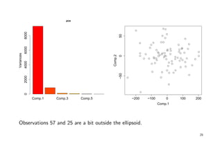
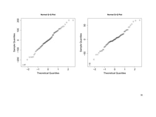
> plot(pca) # or screeplot(pca)
> plot(pca$scores[ , 1:2])
> identify(qqnorm(pca$scores[, 1])); identify(qqnorm(pca$scores[, 2]))
28](https://image.slidesharecdn.com/multivriada-pptms-191117115606/85/Multivriada-ppt-ms-28-320.jpg)
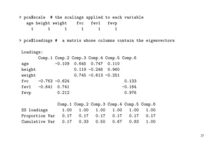
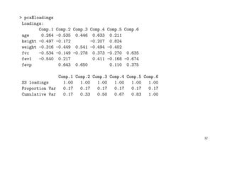
![If we base the analysis on the sample correlation matrix, we get
> pca <- princomp(aimu[ , 3:8], cor=TRUE)
> summary(pca)
Importance of components:
Comp.1 Comp.2 Comp.3 Comp.4 Comp.5 Comp.6
Standard deviation 1.69 1.23 0.91 0.685 0.584 0.0800
Proportion of Variance 0.47 0.25 0.14 0.078 0.057 0.0011
Cumulative Proportion 0.47 0.73 0.86 0.942 0.999 1.0000
> pca$center
age height weight fvc fev1 fevp
30 177 77 553 460 83
> pca$scale
age height weight fvc fev1 fevp
10.4 6.7 10.4 75.8 65.5 6.4
31](https://image.slidesharecdn.com/multivriada-pptms-191117115606/85/Multivriada-ppt-ms-31-320.jpg)


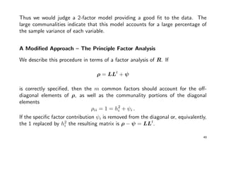
![Example: In a consumer-preference study, a number of customers were asked to
rate several attributes of a new product. The correlation matrix of the responses
was calculated.
Taste 1.00 0.02 0.96 0.42 0.01
Good buy for money 0.02 1.00 0.13 0.71 0.85
Flavor 0.96 0.13 1.00 0.50 0.11
Suitable for snack 0.42 0.71 0.50 1.00 0.79
Provides lots of energy 0.01 0.85 0.11 0.79 1.00
> library(mva)
> R <- matrix(c(1.00,0.02,0.96,0.42,0.01,
0.02,1.00,0.13,0.71,0.85,
0.96,0.13,1.00,0.50,0.11,
0.42,0.71,0.50,1.00,0.79,
0.01,0.85,0.11,0.79,1.00), 5, 5)
> eigen(R)
$values
[1] 2.85309042 1.80633245 0.20449022 0.10240947 0.03367744
46](https://image.slidesharecdn.com/multivriada-pptms-191117115606/85/Multivriada-ppt-ms-46-320.jpg)
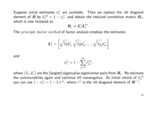
![$vectors
[,1] [,2] [,3] [,4] [,5]
[1,] 0.3314539 0.60721643 0.09848524 0.1386643 0.701783012
[2,] 0.4601593 -0.39003172 0.74256408 -0.2821170 0.071674637
[3,] 0.3820572 0.55650828 0.16840896 0.1170037 -0.708716714
[4,] 0.5559769 -0.07806457 -0.60158211 -0.5682357 0.001656352
[5,] 0.4725608 -0.40418799 -0.22053713 0.7513990 0.009012569
The first 2 eigenvalues of R are the only ones being larger than 1. These two will
account for
2.853 + 1.806
5
= 0.93
of the total (standardized) sample variance. Thus we decide to set m = 2.
There is no special function available in R allowing to get the estimated factor
loadings, communalities, and specific variances (uniquenesses). Hence we directly
calculate those quantities.
47](https://image.slidesharecdn.com/multivriada-pptms-191117115606/85/Multivriada-ppt-ms-47-320.jpg)
![> L <- matrix(rep(0, 10), 5, 2) # factor loadings
> for (j in 1:2) L[ ,j] <- sqrt(eigen(R)$values[j]) * eigen(R)$vectors[ ,j]
[,1] [,2]
[1,] 0.560 0.816
[2,] 0.777 -0.524
[3,] 0.645 0.748
[4,] 0.939 -0.105
[5,] 0.798 -0.543
> h2 <- diag(L %*% t(L)); h2 # communalities
[1] 0.979 0.879 0.976 0.893 0.932
> psi <- diag(R) - h2; psi # specific variances
[1] 0.0205 0.1211 0.0241 0.1071 0.0678
> R - (L %*% t(L) + diag(psi)) # residuals
[,1] [,2] [,3] [,4] [,5]
[1,] 0.0000 0.013 -0.0117 -0.020 0.0064
[2,] 0.0126 0.000 0.0205 -0.075 -0.0552
[3,] -0.0117 0.020 0.0000 -0.028 0.0012
[4,] -0.0201 -0.075 -0.0276 0.000 -0.0166
[5,] 0.0064 -0.055 0.0012 -0.017 0.0000
48](https://image.slidesharecdn.com/multivriada-pptms-191117115606/85/Multivriada-ppt-ms-48-320.jpg)
![Example cont’ed:
> h2 <- 1 - 1/diag(solve(R)); h2 # initial guess
[1] 0.93 0.74 0.94 0.80 0.83
> R.r <- R; diag(R.r) <- h2
> L.star <- matrix(rep(0, 10), 5, 2) # factor loadings
> for (j in 1:2) L.star[ ,j] <- sqrt(eigen(R.r)$values[j]) * eigen(R.r)$vectors[ ,j]
> h2.star <- diag(L.star %*% t(L.star)); h2.star # communalities
[1] 0.95 0.76 0.95 0.83 0.88
> # apply 3 times to get convergence
> R.r <- R; diag(R.r) <- h2.star
> L.star <- matrix(rep(0, 10), 5, 2) # factor loadings
> for (j in 1:2) L.star[ ,j] <- sqrt(eigen(R.r)$values[j]) * eigen(R.r)$vectors[ ,j]
> h2.star <- diag(L.star %*% t(L.star)); h2.star # communalities
[1] 0.97 0.77 0.96 0.83 0.93
51](https://image.slidesharecdn.com/multivriada-pptms-191117115606/85/Multivriada-ppt-ms-51-320.jpg)
![> L.star # loadings
[,1] [,2]
[1,] -0.60 -0.78
[2,] -0.71 0.51
[3,] -0.68 -0.71
[4,] -0.90 0.15
[5,] -0.77 0.58
> 1 - h2.star # specific variances
[1] 0.032 0.231 0.039 0.167 0.069
The principle components method for R can be regarded as a principal factor
method with initial communality estimates of unity (or specific variance estimates
equal to zero) and without iterating.
The only estimating procedure available in R is the maximum likelihood method.
Beside the PCA method this is the only one, which is strongly recommended and
shortly discussed now.
52](https://image.slidesharecdn.com/multivriada-pptms-191117115606/85/Multivriada-ppt-ms-52-320.jpg)
![Maximum Likelihood Method
We now assume that the common factors F and the specific factors are from a
normal distribution. Then maximum likelihood estimates of the unknown factor
loadings L and the specific variances ψ may be obtained.
This strategy is the only one which is implemented in R and is now applied onto
our example.
Example cont’ed:
> factanal(covmat = R, factors=2)
Call:
factanal(factors = 2, covmat = R, rotation = "none")
Uniquenesses: [1] 0.028 0.237 0.040 0.168 0.052
Loadings:
53](https://image.slidesharecdn.com/multivriada-pptms-191117115606/85/Multivriada-ppt-ms-53-320.jpg)
![Factor1 Factor2
[1,] 0.976 -0.139
[2,] 0.150 0.860
[3,] 0.979
[4,] 0.535 0.738
[5,] 0.146 0.963
Factor1 Factor2
SS loadings 2.24 2.23
Proportion Var 0.45 0.45
Cumulative Var 0.45 0.90
54](https://image.slidesharecdn.com/multivriada-pptms-191117115606/85/Multivriada-ppt-ms-54-320.jpg)
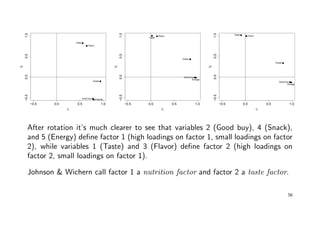
![Factor Rotation
Since the original factor loadings are (a) not unique, and (b) usually not
interpretable, we rotate them until a simple structure is achieved.
We concentrate on graphical methods for m = 2. A plot of the pairs of factor
loadings (ˆi1, ˆi2), yields p points, each point corresponding to a variable. These
points can be rotated by using either the varimax or the promax criterion.
Example cont’ed: Estimates of the factor loadings from the principal component
approach were:
> L
[,1] [,2]
[1,] 0.560 0.816
[2,] 0.777 -0.524
[3,] 0.645 0.748
[4,] 0.939 -0.105
[5,] 0.798 -0.543
> varimax(L)
[,1] [,2]
[1,] 0.021 0.989
[2,] 0.937 -0.013
[3,] 0.130 0.979
[4,] 0.843 0.427
[5,] 0.965 -0.017
> promax(L)
[,1] [,2]
[1,] -0.093 1.007
[2,] 0.958 -0.124
[3,] 0.019 0.983
[4,] 0.811 0.336
[5,] 0.987 -0.131
55](https://image.slidesharecdn.com/multivriada-pptms-191117115606/85/Multivriada-ppt-ms-55-320.jpg)
![Example: A factor analytic analysis of the fvc data might be as follows:
• calculate the maximum likelihood estimates of the loadings w/o rotation,
• apply a varimax rotation on these estimates and check plot of the loadings,
• estimate factor scores and plot them for the n observations.
> fa <- factanal(aimu[, 3:8], factors=2, scores="none", rotation="none"); fa
Uniquenesses:
age height weight VC FEV1 FEV1.VC
0.782 0.523 0.834 0.005 0.008 0.005
Loadings:
Factor1 Factor2
age -0.378 -0.274
height 0.682 -0.109
weight 0.378 -0.153
VC 0.960 -0.270
FEV1 0.951 0.295
FEV1.VC 0.993
58](https://image.slidesharecdn.com/multivriada-pptms-191117115606/85/Multivriada-ppt-ms-58-320.jpg)
![Factor1 Factor2
SS loadings 2.587 1.256
Proportion Var 0.431 0.209
Cumulative Var 0.431 0.640
> L <- fa$loadings
> Lv <- varimax(fa$loadings); Lv
$loadings
Factor1 Factor2
age -0.2810 -0.37262
height 0.6841 0.09667
weight 0.4057 -0.03488
VC 0.9972 0.02385
FEV1 0.8225 0.56122
FEV1.VC -0.2004 0.97716
$rotmat
[,1] [,2]
[1,] 0.9559 0.2937
[2,] -0.2937 0.9559
59](https://image.slidesharecdn.com/multivriada-pptms-191117115606/85/Multivriada-ppt-ms-59-320.jpg)
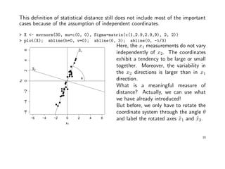
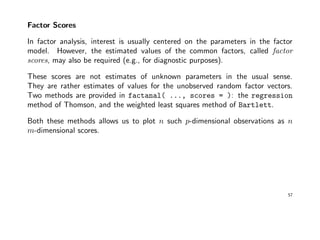
![> plot(L); plot(Lv)
−0.5 0.0 0.5 1.0
−0.50.00.51.0
l1
l2
age
height
weight
VC
FEV1
FEV1.VC
−0.5 0.0 0.5 1.0
−0.50.00.51.0
l1
l2
age
height
weight
VC
FEV1
FEV1.VC
> s <- factanal(aimu[, 3:8], factors=2, scores="reg", rot="varimax")$scores
> plot(s); i <- identify(s, region); aimu[i, ]
60](https://image.slidesharecdn.com/multivriada-pptms-191117115606/85/Multivriada-ppt-ms-60-320.jpg)

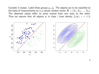


![Example: Fisher’s Iris data
Data describing the sepal (Kelchblatt) width and length, and the petal (Bltenblatt)
width and length of 3 different Iris species (Setosa, Versicolor, Virginica) were
observed. There are 50 observation for each species.
> library(MASS)
> data(iris3)
> Iris <- data.frame(rbind(iris3[,,1], iris3[,,2], iris3[,,3]),
Sp = rep(c("s","c","v"), rep(50,3)))
> z <- lda(Sp ~ Sepal.L.+Sepal.W.+Petal.L.+Petal.W., Iris, prior = c(1,1,1)/3)
Prior probabilities of groups:
c s v
0.3333333 0.3333333 0.3333333
Group means:
Sepal.L. Sepal.W. Petal.L. Petal.W.
c 5.936 2.770 4.260 1.326
s 5.006 3.428 1.462 0.246
v 6.588 2.974 5.552 2.026
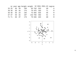
70](https://image.slidesharecdn.com/multivriada-pptms-191117115606/85/Multivriada-ppt-ms-70-320.jpg)
![Coefficients of linear discriminants:
LD1 LD2
Sepal.L. -0.8293776 0.02410215
Sepal.W. -1.5344731 2.16452123
Petal.L. 2.2012117 -0.93192121
Petal.W. 2.8104603 2.83918785
Proportion of trace:
LD1 LD2
0.9912 0.0088
> predict(z, Iris)$class
[1] s s s s s s s s s s s s s s s s s s s s s s s s s s s s s s s
[32] s s s s s s s s s s s s s s s s s s s c c c c c c c c c c c c
[63] c c c c c c c c v c c c c c c c c c c c c v c c c c c c c c c
[94] c c c c c c c v v v v v v v v v v v v v v v v v v v v v v v v
[125] v v v v v v v v v c v v v v v v v v v v v v v v v v
71](https://image.slidesharecdn.com/multivriada-pptms-191117115606/85/Multivriada-ppt-ms-71-320.jpg)
![> table(predict(z, Iris)$class, Iris$Sp)
c s v
c 48 0 1
s 0 50 0
v 2 0 49
> train <- sample(1:150, 75); table(Iris$Sp[train])
c s v
24 25 26
> z1 <- lda(Sp ~ Sepal.L.+Sepal.W.+Petal.L.+Petal.W., Iris,
prior = c(1,1,1)/3, subset = train)
> predict(z1, Iris[-train, ])$class
[1] s s s s s s s s s s s s s s s s s s s s s s s s s c c c c c c
[32] c c c c c c v c c c c c c c c c c c c c v v v v v v v v v v v
[63] v v v c v v v v v v v v v
> table(predict(z1, Iris[-train, ])$class, Iris[-train, ]$Sp)
c s v
c 25 0 1
s 0 25 0
v 1 0 23
72](https://image.slidesharecdn.com/multivriada-pptms-191117115606/85/Multivriada-ppt-ms-72-320.jpg)
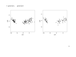
![> ir.ld <- predict(z, Iris)$x # => LD1 and LD2 coordinates
> eqscplot(ir.ld, type="n", xlab="First LD", ylab="Second LD") # eq. scaled axes
> text(ir.ld, as.character(Iris$Sp)) # plot LD1 vs. LD2
> # calc group-spec. means of LD1 & LD2
> tapply(ir.ld[ , 1], Iris$Sp, mean)
c s v
1.825049 -7.607600 5.782550
> tapply(ir.ld[ , 2], Iris$Sp, mean)
c s v
-0.7278996 0.2151330 0.5127666
> # faster alternative:
> ir.m <- lda(ir.ld, Iris$Sp)$means; ir.m
LD1 LD2
c 1.825049 -0.7278996
s -7.607600 0.2151330
v 5.782550 0.5127666
> points(ir.m, pch=3, mkh=0.3, col=2) # plot group means as "+"
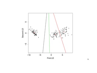
74](https://image.slidesharecdn.com/multivriada-pptms-191117115606/85/Multivriada-ppt-ms-74-320.jpg)
![> perp <- function(x, y, ...) {
+ m <- (x+y)/2 # midpoint of the 2 group means
+ s <- -(x[1]-y[1])/(x[2]-y[2]) # perpendicular line through midpoint
+ abline(c(m[2]-s*m[1], s), ...) # draw classification regions
+ invisible()
> }
> perp(ir.m[1,], ir.m[2,], col=1) # classification decision b/w groups 1&2
> perp(ir.m[1,], ir.m[3,], col=2) # classification decision b/w groups 1&3
> perp(ir.m[2,], ir.m[3,], col=3) # classification decision b/w groups 2&3
75](https://image.slidesharecdn.com/multivriada-pptms-191117115606/85/Multivriada-ppt-ms-75-320.jpg)

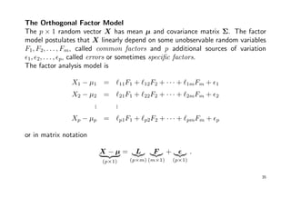
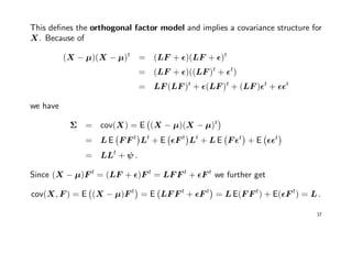
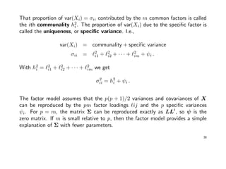
- The document discusses multivariate statistical analysis techniques including principal component analysis (PCA) and factor analysis. - PCA involves identifying linear combinations of original variables that maximize variance and are uncorrelated. The first principal component explains the most variance, followed by subsequent components. - PCA transforms the data to a new coordinate system defined by the eigenvectors of the covariance matrix to extract important information from the data in a lower dimensional representation.


![7.__Developing_a_Research_Proposal[1].pptx](https://cdn.slidesharecdn.com/ss_thumbnails/7-260131073037-df92dd7d-thumbnail.jpg?width=640&height=640&fit=bounds)


![제 23회 보아즈(BOAZ) 빅데이터 컨퍼런스 - [MBOAX] : ABSA를 활용한 소비자 반응 분석 기반 운영 효율화 대시보드 설계](https://cdn.slidesharecdn.com/ss_thumbnails/3-1boaz23rdconferencemboax-260203102709-9d519923-thumbnail.jpg?width=640&height=640&fit=bounds)


