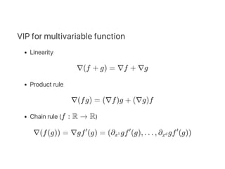
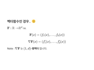
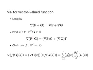
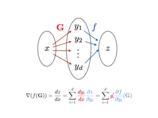
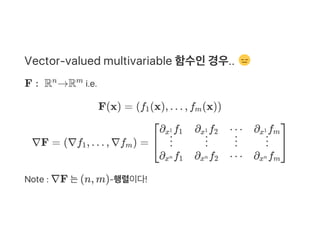
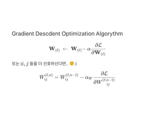
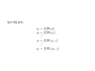
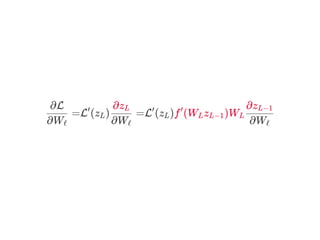
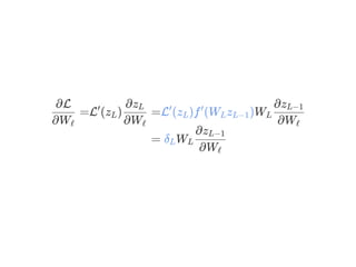
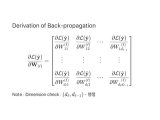
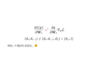
The document serves as a tutorial on linear algebra and matrix calculus, covering essential concepts such as differentiation, matrix operations, and their applications in linear regression and backpropagation in deep learning. It details the mathematical foundations required for understanding multivariable functions, gradients, and optimization techniques including the least squares method. Additionally, it explains the mechanisms of backpropagation for neural networks with emphasis on vectorized operations.
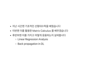


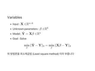
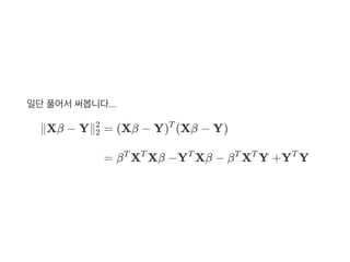
![최소값을구하려면또미분해야합니다!
∇ ∥Xβ − Y∥β 2
2
= ∇ (Xβ) Xβ − (X Y) β − β X Y +Y Yβ ( T T T T T T
)
= ∇ Xβ Xβ + ∇ Xβ Xβ − (X Y) −X Yβ [ ] β [ ] T T
= 2X Xβ − 2X Y = 0T T](https://image.slidesharecdn.com/matrixcalculus-170403100722/85/Matrix-calculus-23-320.jpg)
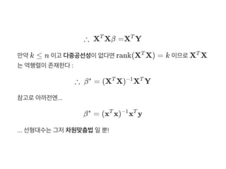
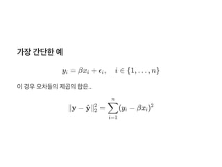
![몇가지쫌센가정이충족된다면 는unbiased, consistent, efficient 한
최적선형추정량(Optimal linear estimator) 이됩니다
= E[Y∣X, β]
Y^
Y^](https://image.slidesharecdn.com/matrixcalculus-170403100722/85/Matrix-calculus-25-320.jpg)
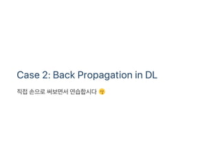
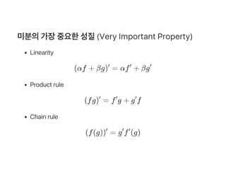
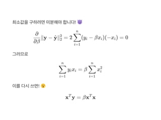
![Loss Function
Mean‑Square Error
L( ∣y) = ∥y − ∥
Cross‑Entropy
L( ∣y) = − [y ⋅ log + (1 − y) ⋅ log(1 − )]
y^
2
1
p∈Batch
∑ p y^p 2
2
y^
dL
1
p∈Batch
∑ y^ y^](https://image.slidesharecdn.com/matrixcalculus-170403100722/85/Matrix-calculus-28-320.jpg)
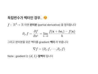
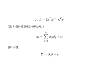
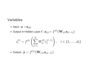
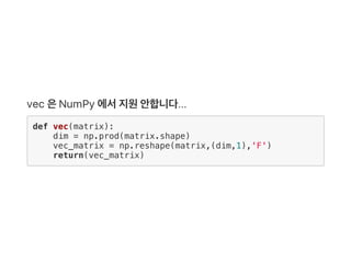
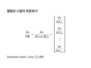
![벡터화연산자
X : (n, m)‑행렬
vec(X) =
X = np.array([[x11,..,x1m],..[xn1,..xnm]]) # (n,m)-행렬
vec_X = np.reshape(X,(nm,1),'F') # (nm,1)-행렬
⎣
⎢
⎢
⎢
⎢
⎢
⎢
⎢
⎢
⎢
⎢
⎡ X11
X21
⋮
Xn1
X12
X22
⋮
Xnm
⎦
⎥
⎥
⎥
⎥
⎥
⎥
⎥
⎥
⎥
⎥
⎤](https://image.slidesharecdn.com/matrixcalculus-170403100722/85/Matrix-calculus-40-320.jpg)
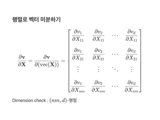

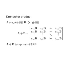
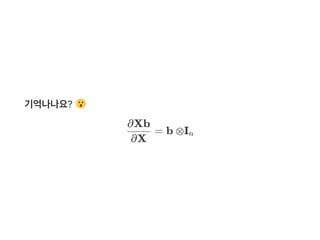
![= b ⊗I
I = np.eye(n) # (n,n)-Identity matrix
b = np.array([[b1],..,[bm]]) # (m,1)-Column vector
np.kron(b,I) # (mn,n)-matrix : Kronecker product
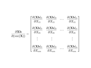
∂X
∂(Xb)
n](https://image.slidesharecdn.com/matrixcalculus-170403100722/85/Matrix-calculus-49-320.jpg)
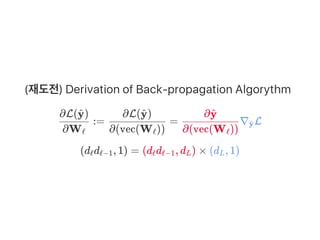
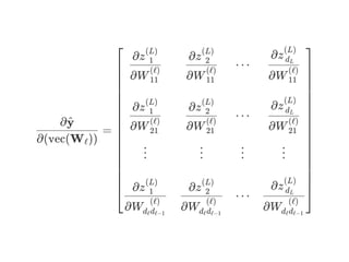
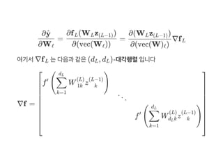
![=
∂(vec(W ))ℓ
∂y^
[
∂(vec(W ))ℓ
∂z 1
(L)
⋯
∂(vec(W ))ℓ
∂z dL
(L)
]](https://image.slidesharecdn.com/matrixcalculus-170403100722/85/Matrix-calculus-51-320.jpg)
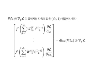
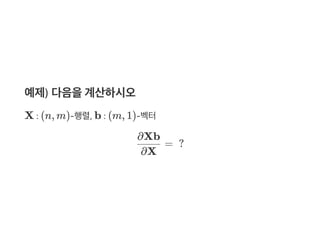
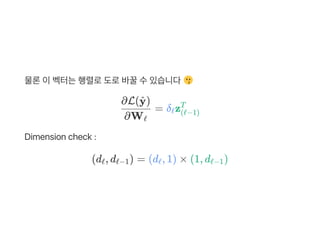
![그러므로... (만약ℓ = L 인경우)
Dimension check :
(d d , 1) = (d d , d ) × (d , 1)
∂WL
∂L( )y^
= diag(∇f ) ⊙ ∇ L
∂(vec(W ))L
∂(W z )L (L−1)
[ L y ]
=z ⊗I δ(L−1) dL L
L L−1 L L−1 L−1 L](https://image.slidesharecdn.com/matrixcalculus-170403100722/85/Matrix-calculus-56-320.jpg)
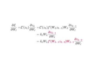
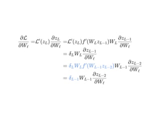
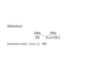
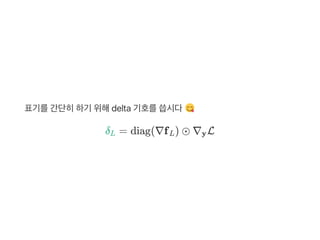
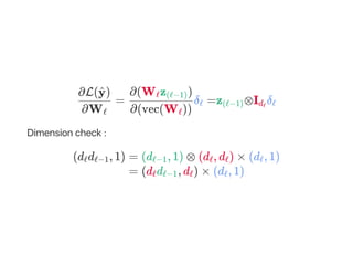
![그러므로... (만약ℓ ≠ L 인경우)
Dimension check :
(d d , d ) × (d , d ) × (d , 1)
∂Wℓ
∂L( )y^
= diag(∇f ) ⊙ ∇ L
∂(vec(W ))ℓ
∂(W z )L (L−1)
[ L y ]
= W δ
∂(vec(W ))ℓ
∂z(L−1)
L
T
L
ℓ ℓ−1 L−1 L−1 L L](https://image.slidesharecdn.com/matrixcalculus-170403100722/85/Matrix-calculus-57-320.jpg)

![뭐한번해보죠...
∂Wℓ
∂L( )y^
= W δ
∂(vec(W ))ℓ
∂z(L−1)
L
T
L
= W δ
∂(vec(W ))ℓ
∂f (W z )L−1 L−1 (L−2)
L
T
L
= diag(∇f ) ⊙W δ
∂(vec(W ))ℓ
∂(W z )L−1 (L−2)
[ L−1 L
T
L]
= W δ
∂(vec(W ))ℓ
∂z(L−2)
L−1
T
L−1](https://image.slidesharecdn.com/matrixcalculus-170403100722/85/Matrix-calculus-59-320.jpg)
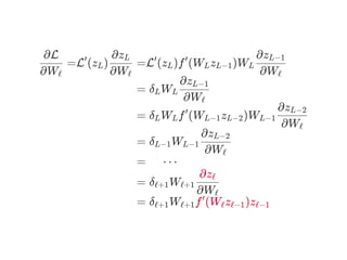
![계속하세요
=
∂Wℓ
∂L( )y^
W δ
∂(vec(W ))ℓ
∂z(L−2)
L−1
T
L−1
= W δ
∂(vec(W ))ℓ
∂f (W z )L−2 L−2 (L−3)
L−1
T
L−1
= diag(∇f ) ⊙W δ
∂(vec(W ))ℓ
∂(W z )L−2 (L−3)
[ L−2 L−1
T
L−1]
= W δ
∂(vec(W ))ℓ
∂z(L−3)
L−2
T
L−2](https://image.slidesharecdn.com/matrixcalculus-170403100722/85/Matrix-calculus-60-320.jpg)
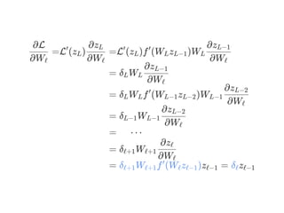
![= ⋯
∂Wℓ
∂L( )y^
= W δ
∂(vec(W ))ℓ
∂zℓ
ℓ+1
T
ℓ+1
= W δ
∂(vec(W ))ℓ
∂f (W z )ℓ ℓ (ℓ−1)
ℓ+1
T
ℓ+1
= diag(∇f ) ⊙W δ
∂(vec(W ))ℓ
∂(W z )ℓ (ℓ−1)
[ ℓ ℓ+1
T
ℓ+1]
= δ
∂(vec(W ))ℓ
∂(W z )ℓ (ℓ−1)
ℓ](https://image.slidesharecdn.com/matrixcalculus-170403100722/85/Matrix-calculus-62-320.jpg)
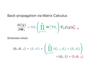
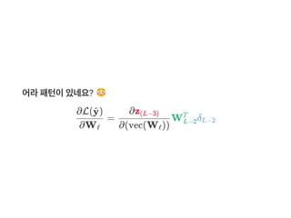
![Back‑propagation Algorythm
위를이용해W , … ,W 를업데이트할수있다
W ← W − α =W − αδ z
δL
δℓ
δ1
= [diag(∇f (W z )) ⊙ ∇ L( )]L L (L−1) y y^
⋮
=W [diag(∇f (W z )) ⊙ δ ]ℓ+1
T
ℓ ℓ (ℓ−1) ℓ+1
⋮
=W [diag(∇f (W x)) ⊙ δ ]2
T
1 1 2
1 L
ℓ ℓ
∂Wℓ
∂L
ℓ ℓ (ℓ−1)
T](https://image.slidesharecdn.com/matrixcalculus-170403100722/85/Matrix-calculus-67-320.jpg)


![[GomGuard] 뉴런부터 YOLO 까지 - 딥러닝 전반에 대한 이야기](https://cdn.slidesharecdn.com/ss_thumbnails/part1mlp2cnn-slidesharev-180308015531-thumbnail.jpg?width=640&height=640&fit=bounds)


![[컴퓨터비전과 인공지능] 6. 역전파 1](https://cdn.slidesharecdn.com/ss_thumbnails/lec6backpropagation-210201173541-thumbnail.jpg?width=640&height=640&fit=bounds)


![[컴퓨터비전과 인공지능] 5. 신경망 2 - 신경망 근사화와 컨벡스 함수](https://cdn.slidesharecdn.com/ss_thumbnails/neuralnetwork2-210128174417-thumbnail.jpg?width=640&height=640&fit=bounds)