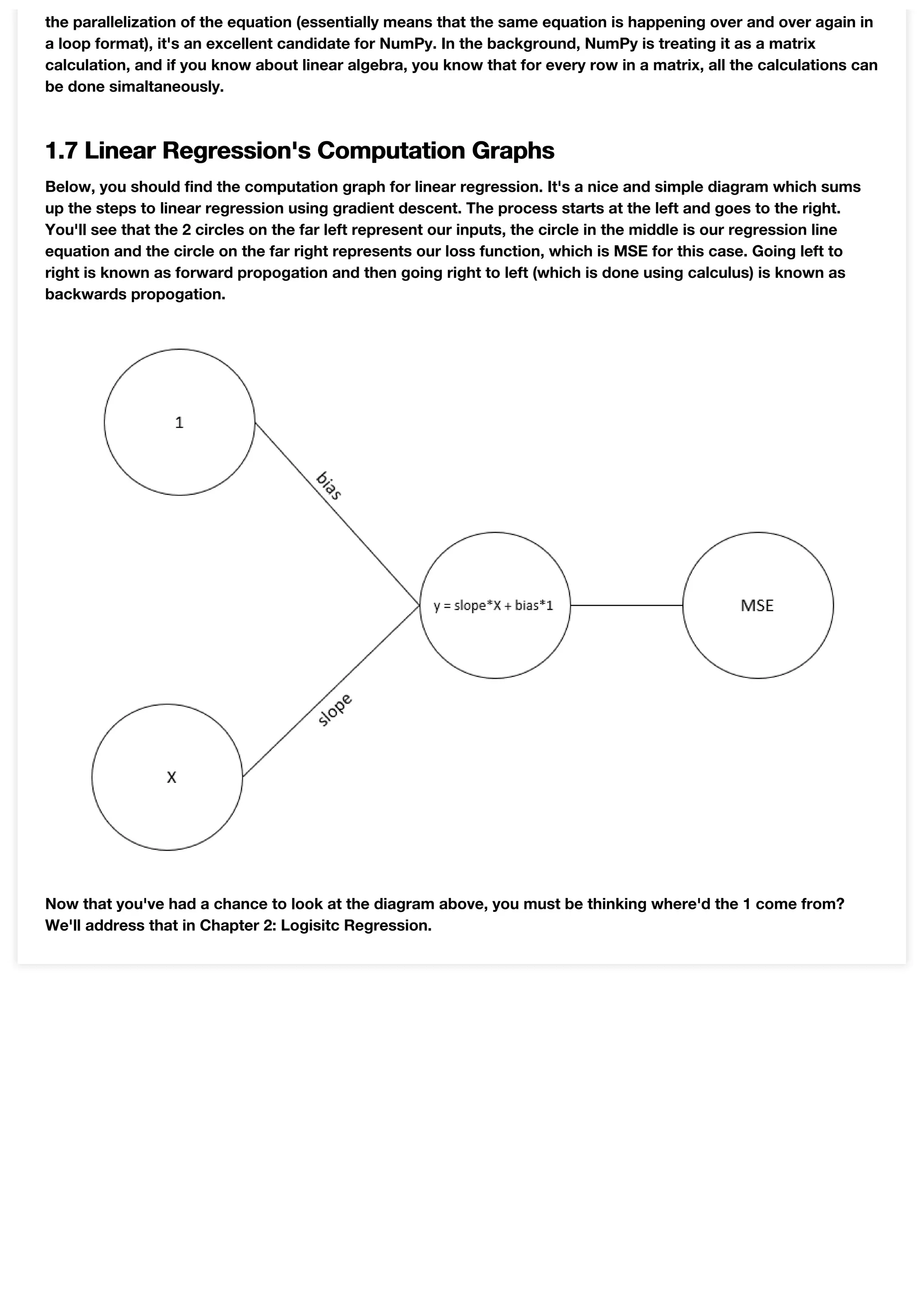
This document provides an introduction and overview of linear regression. It begins by explaining what linear regression is using an example of drawing a best fit line through scatter plot data points. It then walks through creating a mock dataset and visualizing it. Next, it demonstrates drawing an initial best fit line by manually choosing slope and bias values. It introduces the mean squared error metric for evaluating fit and uses it to iteratively improve the line. Finally, it derives the gradient descent algorithm for automatically finding the optimal slope and bias values that minimize mean squared error, without manual adjustment of the parameters. Key steps include calculating partial derivatives of the loss function with respect to slope and bias, then updating the parameters in each iteration based on these gradients.
![Linear Regression
For our very first lesson, we'll go over something called linear regression. What is it exactly? Linear regression is
just a fancy term for something which you probably somewhat already covered in highschool. Do you remember
best fit lines in highschool math? It was you trying to estimate and draw a straight line through a bunch of
points. These points were plotted on a graph and were arranged in a way which appeard that they were going in
the same direction. I hope you're going "oh yeah, I remember that!" Because that's linear regression! Let's go
through it with some code...
1.1 Making a Mock Dataset
Before we start, let's import a couple libraries which we'll use to create our mock dataset. Sklearn (short for
scikit-learn) is a very widely used machine learning library in Python. We won't be covering it in this book, but it
has a nice built-in function (specifically it's "make_regression" function) for easily making mock datasets. As for
matplotlib, it's an easy to use barebones data science library in Python to plot graphs.
In [1]:
from sklearn.datasets import make_regression
import matplotlib.pyplot as plt
Now that we've imported the libraries, let's use sklearn's make_regression function to make our mock dataset.
Don't worry too much about the details regarding the arguments being passed to the function. All you need to
know is that we're going to make 100 mock data points. Each point has a distinct x and y coordinate.
In [2]:
X, Y = make_regression(n_samples=100, n_features=1, bias=5, noise=5, random_state=762)
Y = Y.reshape(-1, 1)
Now that we have our mock data, let's use matplotlib to visualize it.
In [3]:
plt.scatter(X, Y)
plt.show()
I'm hoping that what you're seeing in the plot above is somewhat what you expected to see. What you're seeing
is 100 distinct points, which all seem to be going in the same direction. If you squint your eyes, you'll see that the
points on the graph somewhat make a shape which looks kind of like a straight line.
1.2 Drawing Our Best Fit Line
Now, it's almost time to draw our best fit line. Before we can do that, let's just quickly go over the definition of a](https://image.slidesharecdn.com/chapter1-linearregression-201006140056/75/Chapter-1-Linear-Regression-2-2048.jpg)
![Now, it's almost time to draw our best fit line. Before we can do that, let's just quickly go over the definition of a
line in math. If you remember from highschool math, a line can be define as y=m*x+b, where m represents the
slope, x represents a position on the x-axis and b represents the bias. If none of that made any sense, that's ok.
Playing with the code below should clear it up. I've started you off with values for m and b, but to really
understand how m and b effect the red line below, make sure you give them different values and re-run the code.
Change the values for m and b individually so that you can see how they effect the line.
In [4]:
m, b = 13, 4
y_pred = []
for x in X:
y_pred.append(m*float(x) + b)
plt.scatter(X, Y)
plt.plot(X, y_pred, 'r')
plt.show()
You'll see in the code above that we're plotting 2 different things - the actual points and the line. The line is
defined by our formula y=m*x+b. We loop over each x value in order to get our y value of the line at that point.
There your have it, linear regression!... Well, kinda...
1.3 Finding the Best Fit
So we kinda sorta found a best fit line above. It was us just guessing random values for m and b which made it
look like the line is going through the points on the graph in a balanced way - in a way which we think represents
the general shape of our data well enough that we can take it to be our "best fit" line.
Now, how would you code it so that all of this happens automatically and your algorithm finds a good best fit
line for you? The way I've done it below is semi-automated. I start with the slope (m) and the bias (b) set to 0 and
then I keep incrementing them during every iteration (epoch) by values, which I randomly chose. I decided to set
my last iteration (epoch) to be at a number, not too high and not too low, which I think gives me a good best fit
line. This time, don't play with the values for the slope and the bias, instead, play with the number of epochs to
see how it effects the output.
Just on the side, I'm importing 2 more libraries which are used for demo purposes only. These libraries (time
and IPython) have nothing to do with the actual algorithm. I placed the functions from these 2 libraries between
comments in the actual algorithm, so that you can ignore that part.
In [5]:
import time
from IPython import display
In [6]:
slope = 0
bias = 0
epochs = 15
for epoch in range(epochs):](https://image.slidesharecdn.com/chapter1-linearregression-201006140056/75/Chapter-1-Linear-Regression-3-2048.jpg)
![y_pred = []
for x in X:
y_pred.append(slope*float(x) + bias)
######demo purpose only#####
display.display(plt.gcf())
display.clear_output(wait=True)
##########plotting##########
plt.scatter(X, Y)
plt.plot(X, y_pred, 'r')
plt.title('slope = {0:.1f}, bias = {1:.1f}'.format(slope, bias))
plt.show()
###################
slope += 1
bias += 0.3
1.4 Mean Squared Error
So far, we've come to realize a couple things. We saw that the slope and the bias are the numbers which
influence the line and that linear regression is synonymous to a best fit line. The question I want you to think
about now is, what is it that you're looking at to determine what is a best fit line? In your mind, what are you
doing? How I'd define it is that you're doing a comparison of the "best fit" line and the points on the graph. The
further away the line is to the points, the less likely that line is to be considered a "best fit" line. Let's look at an
example. Run the 2 cells below to output the graphs used for this example.
In [7]:
m, b = 14, 4
y_pred = []
for x in X:
y_pred.append(m*float(x) + b)
plt.scatter(X, Y)
plt.plot(X, y_pred, 'r')
plt.title('Figure 1.4.1')
plt.show()](https://image.slidesharecdn.com/chapter1-linearregression-201006140056/75/Chapter-1-Linear-Regression-4-2048.jpg)
![In [8]:
m, b = 14, -15
y_pred = []
for x in X:
y_pred.append(m*float(x) + b)
plt.scatter(X, Y)
plt.plot(X, y_pred, 'r')
plt.title('Figure 1.4.2')
plt.show()
Looking at Figure 1.4.1 and Figure 1.4.2, which would you deem to be a better fit? Figure 1.4.1 is clearly the
better fit. Why? Because, in general, it's closer to the points.
Is there a mathematical way to get one number to see how far, on average, the line is to the points? Yes, there is!
We're going to use something known as a loss function. That loss function we'll being using for linear regression
is the mean squared error (MSE). For each point, it finds the distance with its respective x value on the line. The
equation does that for all the points and then gets the average.
Let's write it out in a function.
In [9]:
def mse(y, y_pred): ## mean squared error
summation = 0. ## variable for holding the sum of the distanc
es
n = y.shape[0] ## get the amount of points
for i in range(n): ## for each point
summation += (y[i]-y_pred[i])**2 ## get the distance between the point and it's
respective x value
## on the "best fit" line and square it
return float(summation/n) ## return the average distance aas 1 number
The above seems all good and well, but a visualization would probably exaplain it better. Run the cell below to
see our MSE in action. The graph on the left is the graph with our regression points and the graph on the right is
the MSE value at each epoch.
In [10]:
epoch_loss = []
slope = 0
bias = 0
for epoch in range(25):
y_pred = []
for x in X:
y_pred.append(slope*float(x) + bias)
loss = mse(Y, y_pred)](https://image.slidesharecdn.com/chapter1-linearregression-201006140056/75/Chapter-1-Linear-Regression-5-2048.jpg)
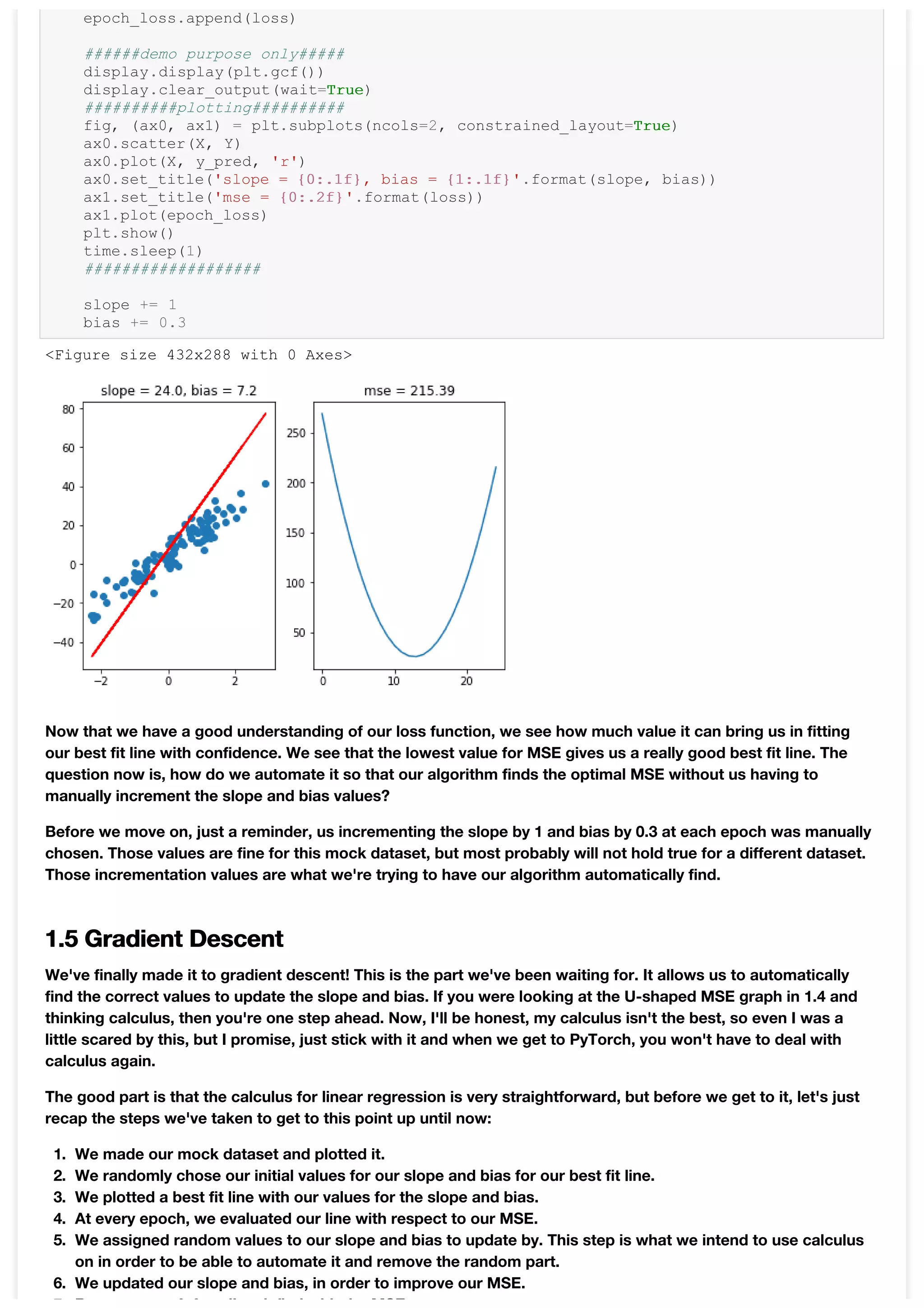
![7. Repeat steps 3-6 until satisfied with the MSE.
If you're still wondering how calculus will help us in our quest to automatically find the lowest MSE, then let's
just take a moment to clarify it. If you remember our MSE graph in 1.4, then you'll remember that the graph
looked like a valley - the optimal value being at the bottom of the valley. Calculus is just a tool to calculate the
slope at a given point. Understanding the steepness of the slope and the direction of it allows us to understand
in what direction we should be heading to be able to get to the bottom of the valley. Us slowly "descending" the
valley is why this process is known as gradient descent.
In this book, we won't cover the rules of calculus, but I do suggest that you go over it, if you haven't alread.
There are many good resources online. Regardless, for the purposes of our exercise, I'll be providing you with
the formulae which would be derived using partial derivates (i.e. calculus).
Starting off, our equation for our MSE is (y-y_pred)^2, where y represents the y-values of our mock dataset and
y_pred represents the y-values for our "best fit" line. The derivative for that ends up to be (y-y_pred).
Now, we get to the equation of our line. We said it is y = (slope * X) + bias. The derivate for the slope ends up
being X and the derivative for the bias ends up being 1.
Putting the derivatives for both equations above together, we end up with 2 equations.
1. The derivative of the MSE with respect to the slope is X * (y-y_pred).
2. The derivative of the MSE with respect to the bias is 1 * (y-y_pred), which is the same as just (y-y_pred).
Awesome! We now have all the equations we need to automatically fit this line, and be sure that it is infact a
best fit for our dataset. Now let's run the cell below and see it in action!
In [11]:
epoch_loss = []
slope = 0.
bias = 0.
learning_rate = 1e-3
n = X.shape[0]
for epoch in range(50):
y_pred = []
for x in X:
y_pred.append(slope*float(x) + bias)
loss = mse(Y, y_pred)
epoch_loss.append(loss)
######demo purpose only#####
display.display(plt.gcf())
display.clear_output(wait=True)
##########plotting##########
fig, (ax0, ax1) = plt.subplots(ncols=2, constrained_layout=True)
fig.suptitle('epoch = {0}'.format(epoch))
ax0.scatter(X, Y)
ax0.plot(X, y_pred, 'r')
ax0.set_title('slope = {0:.1f}, bias = {1:.1f}'.format(slope, bias))
ax1.set_title('mse = {0:.2f}'.format(loss))
ax1.plot(epoch_loss)
plt.show()
time.sleep(1)
###################
###derivatives of mse with respect to slope and bias###
###zero-ing out the gradients###
D_mse_wrt_slope = 0.
D_mse_wrt_bias = 0.
###performing back propagtion for each point on the graph###
for i in range(n):
D_mse_wrt_slope += float(X[i]) * (float(Y[i]) - float(y_pred[i]))
D_mse_wrt_bias += float(Y[i]) - float(y_pred[i])](https://image.slidesharecdn.com/chapter1-linearregression-201006140056/75/Chapter-1-Linear-Regression-7-2048.jpg)
![###updating the slope and bias###
slope += learning_rate * D_mse_wrt_slope
bias += learning_rate * D_mse_wrt_bias
Wow, that was cool! We could have probably stopped at 20 epochs, but I wanted to show how robust our
calculations actually are. No matter how many epochs you go for, it just keeps getting better and better. The
power of math. Who knew all those highschool math courses were actually worth something?
You're probably looking at the code and realizing a few things. The first thing is that there's a variable added
known as the learning_rate. What is that? So remeber I told you that calculus allows us to find out the how steep
the slope is at a given point and hence guides us in descending down to the valley? Well, the learning rate is just
a number which tells our algorithm how big the step should be in our desired direction. It let's our algorithm
know if we should be tip toeing down the slope, or if we should be running down.
Try different values for the learning rate and re-run the cell to see how it effects our algorithm. Try the value 1e-2
and then try 1e-4. Also, how did I come up with 1e-3? Unfortunately, I lied and not everything is 100% automated.
That value was chosen via trial and error, but incrementing/decrementing with 10 to the power of a number is a
good rule to go by.
The other thing you're probably seeing is that we set the partial derivate variables (i.e. gradients) to 0 during
every epoch. This is an important step to make sure your gradients are adding up. Try removing that and seeing
how it effects the algorithm
1.6 No Loops!
So far in this chapter, we've used loops to do our summations. We've also used loops to calculate our y values
for our regression line (i.e. best fit line). A little secret about machine learning practitioners is that we hate loops.
We try every trick in the book to get away from loops. Why? Because it's computationally expensive and it's not
parallelizable.
In order to get away from loops, we're going to import a famous library known as NumPy. It's a very powerful
library used for linear algebra.
In [12]:
import numpy as np
Now that we've imported it, let's rewrite our MSE function using NumPy.
In [13]:
def mse(y, y_pred): ##mean squared error
return np.sum((y - y_pred)**2)/y.shape[0]
That's it! Using NumPy's sum function, we were able to reduce our summation loop into only 1 line!
<Figure size 432x288 with 0 Axes>](https://image.slidesharecdn.com/chapter1-linearregression-201006140056/75/Chapter-1-Linear-Regression-8-2048.jpg)
![That's it! Using NumPy's sum function, we were able to reduce our summation loop into only 1 line!
Let's see how we can implement the rest of the code using NumPy and remove the loops.
In [14]:
epoch_loss = []
slope = 0.
bias = 0.
learning_rate = 1e-3
for epoch in range(50):
##changed##
y_pred = slope*X + bias
###########
loss = mse(Y, y_pred)
epoch_loss.append(loss)
######demo purpose only#####
display.display(plt.gcf())
display.clear_output(wait=True)
##########plotting##########
fig, (ax0, ax1) = plt.subplots(ncols=2, constrained_layout=True)
fig.suptitle('epoch = {0}'.format(epoch))
ax0.scatter(X, Y)
ax0.plot(X, y_pred, 'r')
ax0.set_title('slope = {0:.1f}, bias = {1:.1f}'.format(slope, bias))
ax1.set_title('mse = {0:.2f}'.format(loss))
ax1.plot(epoch_loss)
plt.show()
time.sleep(1)
###################
###derivatives of mse with respect to slope and bias###
##changed##
D_mse_wrt_slope = np.sum(X * (Y - y_pred))
D_mse_wrt_bias = np.sum(Y - y_pred)
###########
slope += learning_rate * D_mse_wrt_slope
bias += learning_rate * D_mse_wrt_bias
Amazing! Without loops, if we don't count the lines used for plotting, we were able to perform linear regression
using gradient descent in only 10 lines!
There's two things I wish to point out before ending this chapter. The first point is that you probably realized that
I'm not explicity zero-ing out the gradients. The reason for that is because we don't need to. Since we're not
using loops anymore, the new values for the gradients just replace the old ones. The second point is that you'll
see that I've also gotten rid of the loop for our regression line equation. How could I do that? Well, because of
<Figure size 432x288 with 0 Axes>](https://image.slidesharecdn.com/chapter1-linearregression-201006140056/75/Chapter-1-Linear-Regression-9-2048.jpg)