1. Legendre Polynomials
• Introduced in 1784 by the French mathematician A. M. Legendre(1752-1833).
• We only study Legendre polynomials which are special cases of Legendre functions. See sections 4.3,
4.7, 4.8, and 4.9 of Kreyszig.
• Legendre functions are important in problems involving spheres or spherical coordinates. Due to their
orthogonality properties they are also useful in numerical analysis.
• Also known as spherical harmonics or zonal harmonics. Called Kugelfunktionen in German. ( Kugel
= Sphere ).
Introduction: Consider Laplace’s equation( see Kreyszig Sec. 8.8 )
2
V =0 (1)
In rectangular coordinates
∂2V ∂2V ∂2V
2
+ 2
+ =0 (2)
∂x ∂y ∂z 2
In spherical coordinates
1 ∂ ∂V 1 ∂ ∂V 1 ∂2V
r2 + sin θ + =0 (3)
r2 ∂r ∂r sin θ ∂θ ∂θ sin2 θ ∂φ2
Equations (2) and (3) express exactly the same fact in different coordinates. Which one to use is a matter
of convenience. Even when spherical coordinates are more natural and equation (3) is used, equation (2)
may give some additional insight due to its greater simplicity.
It is easy to verify that V = 1/r = 1/ x2 + y 2 + z 2 , the potential due to a point source(charge or mass),
satisfies (2) or equivalently (3). This solution is spherically symmetric. Are there solutions which depend on
θ and φ?
One approach to create new solutions from V = 1/r is to take partial derivatives of this function with
respect to x, y, or z. In fact, since ∂/∂x, ∂/∂y, and ∂/∂z operators commute, equation (2) shows that partial
derivatives of all orders of V = 1/r also satisfy the Laplace equation. Let us consider the partial derivatives
of 1/r with respect to z. This will lead us to the Legendre polynomials. (If we consider partial derivatives
with respect to x and y, we will encounter the Associated Legendre functions.)
Some equations relating (x, y, z) to (r, θ, φ) are,
x = r sin θ cos φ (4)
y = r sin θ sin φ (5)
z = r cos θ (6)
r2 = x2 + y 2 + z 2 (7)
From (7) it follows that
∂r z
= (8)
∂z r
Let V = 1/r. Then the first few partial derivatives of V with respect to z are
∂V ∂(1/r) 1 ∂r z cos θ
= =− 2 =− 3 =− 2
∂z ∂z r ∂z r r
∂2V 3z 2 − r2 3 cos2 θ − 1
2
= 5
=
∂z r r3
∂3V 15z 3 − 9zr2 15 cos3 θ − 9 cos θ
3
=− 7
=−
∂z r r4
We notice that ∂ n V /∂z n is an n-th degree polynomial of cos θ divided by rn+1 . One formula which combines
all partial derivatives of V with respect to z is
∂V 1 ∂2V (−1)n ∂ n V
V (x, y, z − h) = V (x, y, z) − h (x, y, z) + h2 2
(x, y, z) + · · · + hn (x, y, z) + · · · (9)
∂z 2! ∂z n! ∂z n
This is just the potential due to a translation of the source, and also satisfies (2), (3).
1

2. Definition: ∞
1 1 hn Pn (cos θ)
=√ = (10)
x2 + y 2 + (z − h)2 r2 − 2rh cos θ + h2 n=0
rn+1
for |h| < r. Equation (10) defines the Legendre polynomial of degree n, Pn . Comparison with (9 ) shows
that
Pn (cos θ) (−1)n ∂ n (1/r)
= (11)
rn+1 n! ∂z n
satisfies the Laplace equation. (This solution of the Laplace equation arises naturally in the study of electric
source configurations known as multipoles. So (10) is actually a multipole potential expansion. Here it
expresses the potential due to a displaced charge in terms of the potentials of multipoles at the origin. The
case n=1 is called a dipole, and the case n=2 is called a quadrupole. In general we have 2n -poles. In fluid
mechanics a doublet is akin to a dipole.) Let w = Pn (cos θ). Then substituting w/rn+1 in (3) in place of V
and simplifying we see that w = Pn (cos θ) satisfies
1 d dw
n(n + 1)w + sin θ =0
sin θ dθ dθ
Or, upon substituting t = cos θ,
d dw
(1 − t2 ) + n(n + 1)w = 0 (12)
dt dt
This is known as Legendre’s differential equation. w = Pn (t) is one of two linearly independent solutions of
this equation. So far we have got the following.
1. A definition of the Legendre polynomials Pn given by (10). We note that (11) can be considered an
equivalent definition.
2. A differential equation (12) which is satisfied by the Legendre polynomials.
In fact, (10) can be written as
∞ ∞
1 1 hn Pn (cos θ) 1
= = (h/r)n Pn (cos θ)
r 1 − 2(h/r) cos θ + (h/r)2 n=0
rn+1 r n=0
Cancelling the 1/r factor, calling h/r as u, and cos θ as t we get the simpler-looking definition
∞
1
√ = un Pn (t) (13)
1 − 2ut + u2 n=0
The left-hand side of (13) is called the generating function of the Legendre polynomials. Many important
properties of the Legendre polynomials can be obtained from (13). We derive several of these properties
now.
Let u = 0 in (13). Then the left-hand side is 1 and the right-hand side is P0 (t). So,
P0 (t) = 1 (14)
√
Let t = 1 in (13). Then the left-hand side is 1/ 1 − 2u + u2 = 1/(1 − u) = 1 + u + u2 + · · ·. The
right-hand side is P0 (1) + uP1 (1) + u2 P2 (1) + · · ·. Comparing the coefficients of un on both sides we get,
Pn (1) = 1 (15)
Substituting t = −1 we can derive,
Pn (−1) = (−1)n (16)
A recurrence relation: Using (11), we get
Pn+1 (cos θ) (−1)n+1 ∂ n+1 (1/r) −1 ∂ Pn (cos θ)
n+2
= n+1
=
r (n + 1)! ∂z n + 1 ∂z rn+1
Or,
Pn+1 (cos θ) −1 (n + 1)Pn (cos θ) ∂r 1 d(Pn (cos θ)) ∂(cos θ)
= − + n+1 (17)
rn+2 n+1 rn+2 ∂z r d cos θ ∂z
2

3. Now
∂r z
= = cos θ (18)
∂z r
What about ∂(cos θ)/∂z? Taking the partial derivative of both sides of (6), that is z = r cos θ, we get
∂r ∂(cos θ) ∂(cos θ) ∂(cos θ)
1= cos θ + r = cos θ. cos θ + r = cos2 θ + r
∂z ∂z ∂z ∂z
So,
∂(cos θ) 1 − cos2 θ
= (19)
∂z r
Using (18) and (19) in (17) we get
Pn+1 (cos θ) −1 (n + 1)Pn (cos θ) 1 d(Pn (cos θ)) 1 − cos2 θ
= − cos θ + n+1
rn+2 n+1 rn+2 r d cos θ r
Cancelling the common 1/rn+2 factor from both sides and simplifying we get
1 − cos2 θ d(Pn (cos θ))
Pn+1 (cos θ) = cos θPn (cos θ) −
n+1 d cos θ
Writing t = cos θ we get,
1 − t2
Pn+1 (t) = tPn (t) − P (t) (20)
n+1 n
where the prime( ) means differentiation with respect to the argument. (20) expresses Pn+1 in terms of
Pn and its derivative. We will use it and the differential equation for Pn to derive several other recurrence
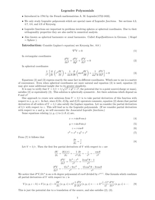
relations later. We use P0 (t) = 1 as a starting condition. Then applying (20) repeatedly we get
P1 (t) = t (21)
3t2 − 1
P2 (t) = (22)
2
5t3 − 3t
P3 (t) = (23)
2
35t4 − 30t2 + 3
P4 (t) = (24)
8
Legendre Polynomials
1 + + + + + + + + + + +
P0 (t) +
P1 (t)
P2 (t)
0.5 P3 (t)
P4 (t)
0
-0.5
-1
-1 -0.5 0 0.5 1
t
Even-odd symmetry: The recurrence (20) also shows that if Pn (t) is an even(odd) function of t then
Pn+1 (t) is an odd(even) function of t. Since P0 is even, it follows that Legendre polynomials of even degrees
are even functions of t, and those of odd degrees are odd functions of t.
3

4. 1
Orthogonality: Now we prove that Pm (t)Pn (t)dt = 0, if integers m ≥ 0 and n ≥ 0 are unequal. Let
−1
v = Pm (t) and w = Pn (t). Then by Legendre’s differential equation (12)
(1 − t2 )v + m(m + 1)v = 0 (25)
(1 − t2 )w + n(n + 1)w = 0 (26)
Now we multiply (25) by w and integrate from t = −1 to t = 1 to obtain
1 1
(1 − t2 )v wdt + m(m + 1) vwdt = 0
−1 −1
Integrating the first integral by parts we get,
1 1
1
(1 − t2 )v w −1
− (1 − t2 )v w dt + m(m + 1) vwdt = 0
−1 −1
But since (1 − t2 ) is zero both at t = −1 and t = 1 this becomes,
1 1
− (1 − t2 )v w dt + m(m + 1) vwdt = 0 (27)
−1 −1
In exactly the same way we can multiply (26) by v and integrate from t = −1 to t = 1 to obtain
1 1
− (1 − t2 )v w dt + n(n + 1) vwdt = 0 (28)
−1 −1
Subtracting (28) from (27) we get
1
(m(m + 1) − n(n + 1)) vwdt = 0
−1
Or, since v = Pm (t) and w = Pn (t)
1
(m(m + 1) − n(n + 1)) Pm (t)Pn (t)dt = 0
−1
This gives the orthogonality relationship:
1
Pm (t)Pn (t)dt = 0 (29)
−1
for m = n, and m ≥ 0, n ≥ 0. This is a very important property of the Legendre polynomials.
1 2
To determine −1 Pn (t)dt we square (13) and integrate from t = −1 to t = 1. Due to orthogonality only
2
the integrals of terms having Pn (t) survive on the right-hand side. So we get
1 ∞ 1
1
dt = u2n 2
Pn (t)dt
−1 1 − 2ut + u2 n=0 −1
Or,
∞ ∞ 1
1 1+u 2u2n
ln = = u2n 2
Pn (t)dt
u 1 − u n=0 2n + 1 n=0 −1
Comparing coefficients of u2n we get
1
2 2
Pn (t)dt = (30)
−1 2n + 1
More recurrences: Rearranging (20) we get
(1 − t2 )Pn (t) = (n + 1)(tPn (t) − Pn+1 (t)) (31)
4

5. Differentiating both sides of (20) with respect to t and using the fact(from (12)) that ((1 − t2 )Pn (t)) =
−n(n + 1)Pn (t) we get after some simplification
Pn+1 (t) = (n + 1)Pn (t) + tPn (t) (32)
Multiplying both sides of (32) by (1 − t2 ) we get
(1 − t2 )Pn+1 (t) = (n + 1)(1 − t2 )Pn (t) + t(1 − t2 )Pn (t)
But since by (31) (1 − t2 )Pn (t) = (n + 1)(tPn (t) − Pn+1 (t))
(1 − t2 )Pn+1 (t) = (n + 1)(1 − t2 )Pn (t) + t(n + 1)(tPn (t) − Pn+1 (t))
On simplification we get
(1 − t2 )Pn+1 (t) = (n + 1)(Pn (t) − tPn+1 (t)) (33)
Rearranging (33) we get
(1 − t2 )
Pn (t) = tPn+1 (t) + P (t) (34)
n + 1 n+1
If in (33) we decrement n by 1 we get
(1 − t2 )Pn (t) = n(Pn−1 (t) − tPn (t)) (35)
Comparing (31) and (35) we get
n(Pn−1 (t) − tPn (t)) = (n + 1)(tPn (t) − Pn+1 (t))
On simplification this gives Bonnet’s recursion formula.
(n + 1)Pn+1 (t) = (2n + 1)tPn (t) − nPn−1 (t) (36)
Since this formula involves no derivatives it is much used in programs to compute the Legendre polynomials.
One usually starts with P0 (t) = 1 and P1 (t) = t.
Location and interlacing of zeros: Plotting Pn (t) for the first few values of n we see that:
1. Between two consecutive zeros of Pn+1 (t) there is one of Pn (t).
2. Between two consecutive zeros of Pn (t) there is one of Pn+1 (t). Between the smallest zero of Pn (t) and
−1 there is one zero of Pn+1 (t). Between the largest zero of Pn (t) and +1 there is one zero of Pn+1 (t).
3. All n zeros of Pn (t) lie in −1 < t < 1.
These statements, which are of great use in the numerical calculation of the zeros of Pn (t), may be proved
using the recurrence relationships derived earlier. A rough sketch of these proofs follows.
To prove the first statement we multiply both sides of (34) by (n + 1)/(1 − t2 )(n+3)/2 to obtain
(n + 1)Pn (t) (n + 1)tPn+1 (t) Pn+1 (t)
2 )(n+3)/2
= 2 )(n+3)/2
+
(1 − t (1 − t (1 − t2 )(n+1)/2
Or,
(n + 1)Pn (t) Pn+1 (t)
= (37)
(1 − t2 )(n+3)/2 (1 − t2 )(n+1)/2
By Rolle’s theorem the first statement follows.
We multiply both sides of (20) by (n + 1)(1 − t2 )(n−1)/2 to obtain
(n + 1)(1 − t2 )(n−1)/2 Pn+1 (t) = (n + 1)t(1 − t2 )(n−1)/2 Pn (t) − (1 − t2 )(n+1)/2 Pn (t)
Or,
(n + 1)(1 − t2 )(n−1)/2 Pn+1 (t) = (−(1 − t2 )(n+1)/2 Pn (t)) (38)
2 (n+1)/2
So, by Rolle’s theorem between two zeros of −(1 − t ) Pn (t) there is at least one of (n + 1)(1 −
t2 )(n−1)/2 Pn+1 (t). But the first function is zero when Pn (t) is zero or when t = −1 or t = +1. This proves
the second statement about the zeros mentioned above. It follows that if Pn (t) has n zeros in (−1, 1), then
Pn+1 (t) has n + 1 zeros in (−1, 1). But it is known that P1 (t), which equals t, has one zero in (−1, 1). Then
using the method of mathematical induction we can prove that Pn (t) has n zeros in (−1, 1) for all integral
n ≥ 0. This proves the third statement.
5