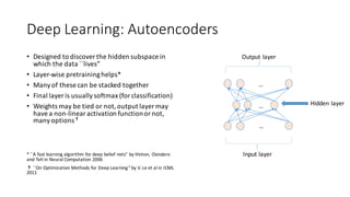
The document provides an overview of classification algorithms in Apache SystemML, including supervised learning techniques like support vector machines, logistic regression, naive Bayes, and decision trees. It discusses how these algorithms are formulated and implemented in SystemML, with a focus on optimization methods and parallelization. Key topics covered include the representer theorem, dual formulations, multi-class extensions, and using group-by aggregates and matrix operations for efficient training.

1. Classification Algorithms in
Apache SystemML
Prithviraj Sen

2. Overview
• Supervised Learning and Classification
• Training Discriminative Classifiers
• Representer Theorem
• Support Vector Machines
• Logistic Regression
• Generative Classifiers: Naïve Bayes
• Deep Learning
• Tree Ensembles

3. Classification and Supervised Learning
• Supervised learning is a major area of machine learning
• Goal is to learn function 𝑓 such that:
𝑓: ℝm → C
where: m is a fixed integer
C is a fixed domain of labels
• Training: goal is to learn 𝑓 from a labeled dataset
• Testing: goal is to apply 𝑓 to unseen x ∈ ℝm
• Applications:
• spam detection (D = {spam, no-spam})
• search advertising (each ad is a label)
• recognizing hand-written digits (D = {0, 1, …, 9})

4. Training a Classifier
• Given labeled training data: {(x1, y1), (x2, y2), …, (xn, yn)}
𝑓 = argmin 𝑓 ∑ ℓ01(𝑓(𝒙𝑖), 𝑦𝑖) /
012
• Multiple issues*:
• We have not chosen a form for 𝑓
• ℓ01 is not convex
ℓ01(u,v) = 3
0 if sign(𝑢) = sign(𝑣)
1 otherwise
* ``Algorithms for Direct 0-1 Loss Optimization in Binary Classification” by Nguyen and Sanner in ICML 2013

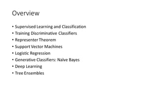
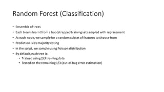
5. Training Discriminative Classifiers
𝑓 = argmin 𝑓 ∑ ℓ(𝑓(𝒙𝑖), 𝑦𝑖) + ℊ(∥ 𝑓 ∥)/
012
• The second term is ``regularization”
• A common form for 𝑓(𝒙) is 𝐰′𝒙 (linear classifier)
• ℓ(w’x,y) is ``convexified” loss
• Besides discriminative classifiers, generative classifiers also exist
• e.g., naïve Bayes
Classifier Loss function (y ∈ {±1})
support vector machine max(0, 1 - y w’x)
logistic regression log[1 + exp(-y w’x)]
adaboost exp(-y w’x)
square loss (1 – y w’x)2
Algorithms for Direct 0–1 Loss Optim
−1.5 −1 −0.5 0 0.5 1 1.5 2
0
1
2
3
4
5
6
7
8
margin (m)
LossValue
0−1 Loss
Hinge Loss
Log Loss
Squared Loss
T
ar
is
W
in
(w
fw
as
th
T
{x
t
cl

6. Representer Theorem*
• If ℊ is real-valued, monotonically increasing and lies in [0,∞)
• And if ℓ lies in ℝ⋃{∞}, then
f(x) = ∑ 𝛼𝑖
𝒙′𝒙𝑖 /
012
• In particular,
• Neither convexity nor differentiability is necessary
• But helps with the optimization
• Especially when using gradient based methods
*``A Generalized Representer Theorem” by Scholkopf, Herbrich and Smola in COLT 2001
☨``When is there a Representer Theorem?” by Argyriou, Micchelli and Pontil in JMLR 2009

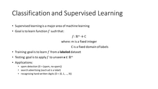
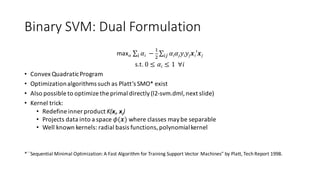
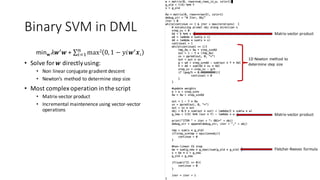
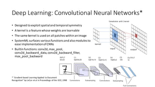
7. Binary Class Support Vector Machines
minw ∑ max 0,1 − 𝑦𝑖𝒘S 𝒙𝑖 +
T
U
𝒘S 𝒘 /
012
• Expressed in standard form:
minw ∑ ξi +
T
U
𝒘S 𝒘 0
s.t. 𝑦𝑖 𝒘S 𝒙𝑖 ≥ 1 − ξi
∀𝑖
ξi ≥ 0 ∀𝑖
• Lagrangian (𝛼𝑖, 𝛽𝑖 ≥ 0):
ℒ = ∑ ξi +
T
U
𝒘S 𝒘 + ∑ 𝛼𝑖(1 − 𝑦𝑖 𝒘S 𝒙𝑖 − ξi00 ) − ∑ 𝛽𝑖 𝜉𝑖0
]ℒ
𝝏w
: w =
2
_
∑ 𝛼𝑖 𝑦𝑖 𝒙𝑖0
]ℒ
𝝏`i
: 1 = 𝛼𝑖+𝛽𝑖 ∀
𝑖

8. Binary SVM: Dual Formulation
max 𝛼 ∑ 𝛼𝑖 0 −
2
U
∑ 𝛼𝑖 𝛼𝑗 𝑦𝑖 𝑦𝑗 𝒙𝑖′𝒙𝑗0b
s.t. 0 ≤ 𝛼𝑖 ≤ 1 ∀𝑖
• Convex Quadratic Program
• Optimization algorithms such as Platt’s SMO* exist
• Also possible to optimize the primal directly (l2-svm.dml, next slide)
• Kernel trick:
• Redefine inner product K(xi, xj)
• Projects data into a space 𝜙(𝒙) where classes may be separable
• Well known kernels: radial basis functions, polynomial kernel
*``Sequential Minimal Optimization: A Fast Algorithm for Training Support Vector Machines” by Platt, Tech Report 1998.

9. Binary SVM in DML
minw 𝜆𝒘S 𝒘 + ∑ max2 0,1 − 𝑦𝑖𝒘S 𝒙𝑖 /
012
• Solve for 𝒘 directly using:
• Non linear conjugate gradient descent
• Newton’s method to determine step size
• Most complex operation in the script
• Matrix-vector product
• Incremental maintenence using vector-vector
operations
Matrix-vector product
Matrix-vector product
Fletcher-Reeves formula
1D Newton method to
determine step size

10. Multi-Class SVM in DML
• At least 3 different ways to define multi-class
SVMs
• One-against-the-rest* (OvA)
• Pairwise (or one-against-one)
• Crammer-Singer SVM☨
• OvA multi-class SVM
• Each binary class SVM learnt in parallel
• Inner body uses l2-svm’s approach
*``In Defense of One-vs-All Classification” by Rifkin and Klautau in
JMLR 2004
☨``On the Algorithmic Implementation of Multiclass Kernel-
Based Vector Machines” by Crammer and Singer in JMLR 2002
…
Parallel for loop

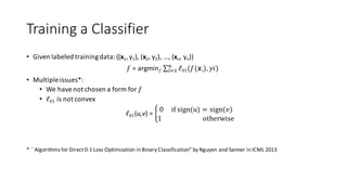
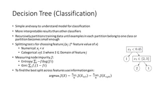
11. Logistic Regression
maxw -∑ log 1 + 𝑒hi0 𝒘j 𝒙0 −
T
U
𝒘S 𝒘 /
012
• To derive the dual form use the following bound*:
log
2
2klmn𝒘j 𝒙
≤ min 𝛼
𝛼𝑦𝒘′𝒙 − 𝐻(𝛼)
where 0 ≤ 𝛼 ≤ 1 and 𝐻(𝛼) = −𝛼log(𝛼) − (1 − 𝛼)log(1 − 𝛼)
• Substituting:
maxw min 𝛼 ∑ 𝛼𝑖 𝑦𝑖 𝒘′𝒙𝑖0 − 𝐻(𝛼𝑖) −
T
U
𝒘S 𝒘 s.t. 0 ≤ 𝛼𝑖 ≤ 1 ∀𝑖
]ℒ
𝝏w
: w =
2
_
∑ 𝛼𝑖 𝑦𝑖 𝒙𝑖0
• Dual form:
min 𝛼
2
UT
∑ 𝛼𝑖 𝛼𝑗 𝑦𝑖 𝑦𝑗 𝒙𝑖′𝒙𝑗0b − ∑ 𝐻(𝛼𝑖)0 s.t. 0 ≤ 𝛼𝑖 ≤ 1 ∀𝑖
• Apply kernel trick to obtain kernelized logistic regression
*``Probabilistic Kernel Regression Models” by Jaakkola and Haussler in AISTATS 1999

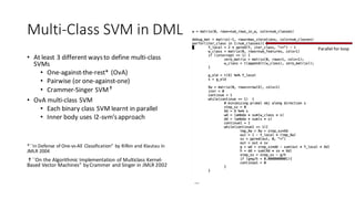
12. Multiclass Logistic Regression
• Also called softmax regression or multinomial logistic regression
• W is now a matrix of weights, jth column contains the jth class’s weights
Pr(y|x) =
lp
j
qn
∑ lp
j
qn
n
minW
_
U
∥ 𝑊 ∥ 2 + ∑ [log(Zi)0 − 𝑥𝑖′𝑊𝑦𝑖] where 𝑍𝑖 = 1S 𝑒wjx0
• The DML script is called MultiLogReg.dml
• Uses trust-region Newton method to learn the weights*
• Care needs to be taken because softmax is an over-parameterized function
*See regression class’s slides on ibm.biz/AlmadenML

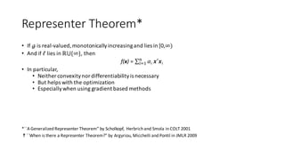
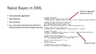
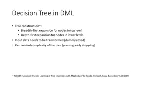
13. Generative Classifiers: Naïve Bayes
• Generative models “explain” the generation of the data
• Naïve Bayes assumes, each feature is independent given class label
Pr(x,y) = py ∏ (𝑝𝑦𝑗b )nj
• A conjugate prior is used to avoid 0 probabilities
Pr({(xi,yi)}) = ∏ [
{|
(_)
{(|_)
∏ 𝑝 𝑦𝑗
𝜆]bi ∏ [𝑝𝑦𝑖∏ 𝑝 𝑦𝑖𝑗
𝑛𝑖𝑗]b0
s.t. 𝑝 𝑦 ∀ 𝑦, 𝑝𝑦𝑗 ∀𝑦 ∀𝑗 form legal distributions
• Maximum is obtained when:
𝑝 𝑦 =
𝑛 𝑦
∑ 𝑛 𝑦i
∀𝑦, 𝑝𝑦𝑗 =
𝜆 + ∑ 𝑛𝑖𝑗0:i01i
𝑚𝜆 + ∑ ∑ 𝑛𝑖𝑗b0:i01i
∀𝑦∀𝑗
• This is multinomial naïve Bayes, other forms include multivariate Bernoulli*
* ``A Comparison of Event Models for Naïve Bayes Text Classification” by McCallum and Nigam in AAAI/ICML-98 Workshop on Learning for Text
Categorization

14. Naïve Bayes in DML
• Uses group by aggregates
• Very efficient
• Non-iterative
• E.g., document classification with term
frequency feature vectors (bag-of-words)
Group by aggregate
Matrix-vector op
Group by count

15. Deep Learning: Autoencoders
• Designed to discover the hidden subspace in
which the data ``lives”
• Layer-wise pretraininghelps*
• Many of these can be stacked together
• Final layer is usually softmax (for classification)
• Weights may be tied or not, output layer may
have a non-linear activation function or not,
many options☨
*``A fast learning algorithm for deep belief nets” by Hinton, Osindero
and Teh in Neural Computation 2006
☨ ``On Optimization Methods for Deep Learning” by V. Le et al in ICML
2011
…
…
…
Input layer
Output layer
Hidden layer

16. Deep Learning: Convolutional Neural Networks*
• Designed to exploit spatial and temporal symmetry
• A kernel is a feature whose weights are learnable
• The same kernel is used on all patches within an image
• SystemML surfaces various functions and also modules to
ease implementation of CNNs
• Builtin functions: conv2d, max_pool,
conv2d_backward_data, conv2d_backward_filter,
max_pool_backward
Convolution with 1 kernel
*``Gradient-based Learning Applied to Document
Recognition” by LeCun et al in Proceedings of the IEEE, 1998

17. Decision Tree (Classification)
• Simple and easy to understand model for classification
• More interpretable results than other classifiers
• Recursively partitions training data until examples in each partition belong to one class or
partition becomes small enough
• Splitting test s for choosing feature j (xj: jth feature value of x)
• Numerical: xj < 𝜎
• Categorical: xj∈ S where S ⊆ Domain of feature j
• Measuring node impurity 𝒥:
• Entropy: ∑ −𝑓𝑖log(𝑓𝑖)0
• Gini: ∑ 𝑓𝑖(1 − 𝑓𝑖)0
• To find the best split across features use information gain:
argmax 𝒥 𝑋 −
/…l†‡
/
𝒥 𝑋𝑙𝑒𝑓𝑡 −
/Š0‹Œ‡
/
𝒥 𝑋 𝑟𝑖𝑔ℎ𝑡

18. Decision Tree in DML
• Tree construction*:
• Breadth-first expansion for nodes in top level
• Depth-first expansion for nodes in lower levels
• Input data needs to be transformed (dummy coded)
• Can control complexity of the tree (pruning, early stopping)
*``PLANET: Massively Parallel Learning of Tree Ensembles with MapReduce” by Panda, Herbach, Basu, Bayardoin VLDB 2009

19. Random Forest (Classification)
• Ensemble of trees
• Each tree is learnt from a bootstrapped training set sampled with replacement
• At each node, we sample for a random subset of features to choose from
• Prediction is by majority voting
• In the script, we sample using Poisson distribution
• By default, each tree is:
• Trained using 2/3 training data
• Tested on the remaining 1/3 (out-of-bag error estimation)