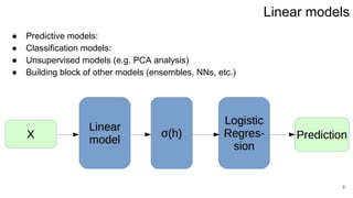
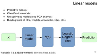
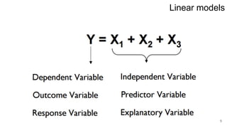
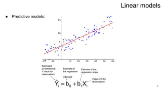
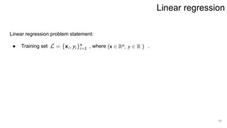
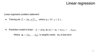
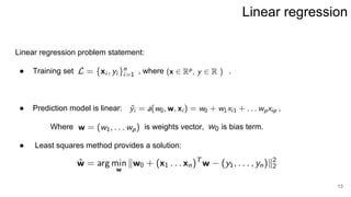
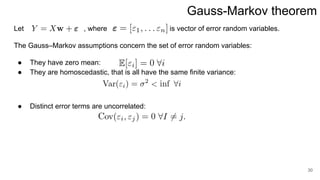
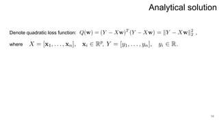
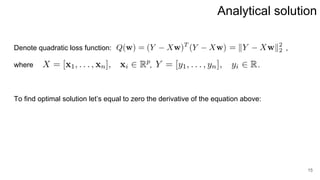
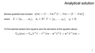
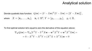
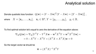
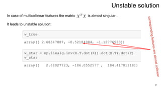
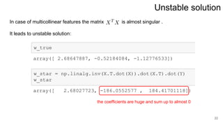
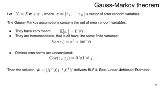
This lecture covers linear regression models. It discusses linear regression problem statements, analytical solutions using least squares, regularization to address ill-conditioned matrices, and probabilistic interpretations of regularization. The key topics are: 1. Linear regression finds a linear function to model the relationship between inputs and output in a dataset. 2. Least squares estimation provides an analytical solution for the optimal weights vector that minimizes error. 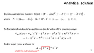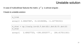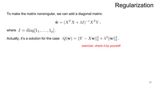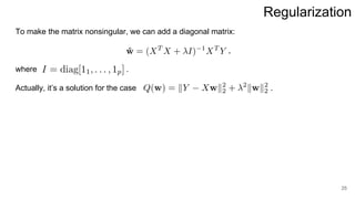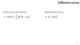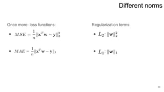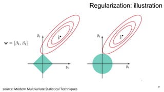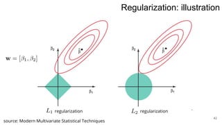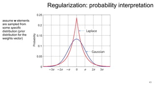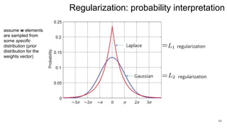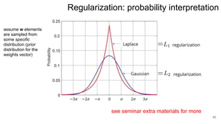3. Regularization adds a diagonal matrix to make the matrix nonsingular when features are multicollinear, providing a more stable solution.

1. Lecture 2: Linear regression
Machine Learning Course
MIPT, 2019

2. 1. Overview of linear models.
2. Linear regression.
3. Analytical solution.
4. Regularization.
5. Gauss-Markov theorem.
6. Probabilistic interpretation and intuition.
Outline
2

3. 3

4. 4
Example questions linear regression can solve (up
right picture):
● What will be my monthly spending for the next
year?
● Which factor is more important in deciding my
monthly spending?
● How monthly income and trips per month are
correlated with monthly spending?

5. 5
Linear models

6. 6
● Predictive models:
Linear models

7. 7
● Predictive models:
● Classification models:
Linear models

8. 8
● Predictive models:
● Classification models:
● Unsupervised models (e.g. PCA analysis)
Linear models

9. 9
● Predictive models:
● Classification models:
● Unsupervised models (e.g. PCA analysis)
● Building block of other models (ensembles, NNs, etc.)
Linear models

10. 10
● Predictive models:
● Classification models:
● Unsupervised models (e.g. PCA analysis)
● Building block of other models (ensembles, NNs, etc.)
Linear models
Actually, it’s a neural network. We will meet it later.

11. 11
Linear regression
Linear regression problem statement:
● Training set , where .

12. 12
Linear regression
Linear regression problem statement:
● Training set , where .
● Prediction model is linear: ,
Where is weights vector, is bias term.

13. 13
Linear regression
Linear regression problem statement:
● Training set , where .
● Prediction model is linear: ,
Where is weights vector, is bias term.
● Least squares method provides a solution:

14. 14
Analytical solution
Denote quadratic loss function: ,
where , .

15. 15
Analytical solution
Denote quadratic loss function: ,
where , .
To find optimal solution let’s equal to zero the derivative of the equation above:

16. 16
Analytical solution
Denote quadratic loss function: ,
where , .
To find optimal solution let’s equal to zero the derivative of the equation above:

17. 17
Analytical solution
Denote quadratic loss function: ,
where , .
To find optimal solution let’s equal to zero the derivative of the equation above:

18. 18
Analytical solution
Denote quadratic loss function: ,
where , .
To find optimal solution let’s equal to zero the derivative of the equation above:
So the target vector w should be

19. 19
Analytical solution
Denote quadratic loss function: ,
where , .
To find optimal solution let’s equal to zero the derivative of the equation above:
So the target vector w should be
what if this matrix is singular?

20. 20
Unstable solution
In case of multicollinear features the matrix is almost singular .
It leads to unstable solution:

21. 21
Unstable solution
In case of multicollinear features the matrix is almost singular .
It leads to unstable solution:

22. 22
Unstable solution
In case of multicollinear features the matrix is almost singular .
It leads to unstable solution:
the coefficients are huge and sum up to almost 0

23. 23
Regularization
To make the matrix nonsingular, we can add a diagonal matrix:
,
where .
Actually, it’s a solution for the case .

24. 24
Regularization
To make the matrix nonsingular, we can add a diagonal matrix:
,
where .
Actually, it’s a solution for the case .
exercise: check it by yourself

25. 25
Regularization
To make the matrix nonsingular, we can add a diagonal matrix:
,
where .
Actually, it’s a solution for the case .

26. Let , where is vector of error random variables.
26
Gauss-Markov theorem

27. Let , where is vector of error random variables.
The Gauss–Markov assumptions concern the set of error random variables:
27
Gauss-Markov theorem

28. 28
Gauss-Markov theorem
Let , where is vector of error random variables.
The Gauss–Markov assumptions concern the set of error random variables:
● They have zero mean:

29. 29
Gauss-Markov theorem
Let , where is vector of error random variables.
The Gauss–Markov assumptions concern the set of error random variables:
● They have zero mean:
● They are homoscedastic, that is all have the same finite variance:

30. 30
Gauss-Markov theorem
Let , where is vector of error random variables.
The Gauss–Markov assumptions concern the set of error random variables:
● They have zero mean:
● They are homoscedastic, that is all have the same finite variance:
● Distinct error terms are uncorrelated:

31. 31
Gauss-Markov theorem
Let , where is vector of error random variables.
The Gauss–Markov assumptions concern the set of error random variables:
● They have zero mean:
● They are homoscedastic, that is all have the same finite variance:
● Distinct error terms are uncorrelated:
Then the solution delivers BLEU: Best Linear Unbiased Estimator.

32. Once more: loss functions:
●
32
Regularization terms:
● :
Different norms

33. Once more: loss functions:
●
●
33
Regularization terms:
● :
● :
Different norms

34. Once more: loss functions:
●
●
34
Regularization terms:
● :
● :
Different norms
only works for Gauss-Markov theorem

35. 35
What’s the difference?

36. 36
What’s the difference?
● MSE
○ delivers BLUE according to
Gauss-Markov theorem
○ differentiable
○ sensitive to noise

37. 37
What’s the difference?
● MSE
○ delivers BLUE according to
Gauss-Markov theorem
○ differentiable
○ sensitive to noise
● MAE
○ non-differentiable
■ (actually, it is differentiable)
○ much more prone to noise

38. 38
What’s the difference?
● MSE
○ delivers BLUE according to
Gauss-Markov theorem
○ differentiable
○ sensitive to noise
● MAE
○ non-differentiable
■ (actually, it is differentiable)
○ much more prone to noise
● regularization
○ constraints weights
○ delivers more stable solution
○ Differentiable

39. 39
What’s the difference?
● MSE
○ delivers BLUE according to
Gauss-Markov theorem
○ differentiable
○ sensitive to noise
● MAE
○ non-differentiable
■ (actually, it is differentiable)
○ much more prone to noise
● regularization
○ constraints weights
○ delivers more stable solution
○ Differentiable
● regularization
○ non-differentiable
■ (actually, the same as MAE ;)
○ selects features

40. 40
What’s the difference?
● MSE
○ delivers BLUE according to
Gauss-Markov theorem
○ differentiable
○ sensitive to noise
● MAE
○ non-differentiable
■ (actually, it is differentiable)
○ much more prone to noise
● regularization
○ constraints weights
○ delivers more stable solution
○ Differentiable
● regularization
○ non-differentiable
■ (actually, the same as MAE ;)
○ selects features
Does what?

41. 41
source: Modern Multivariate Statistical Techniques
Regularization: illustration

42. 42
source: Modern Multivariate Statistical Techniques
regularization regularization
Regularization: illustration

43. 43
Regularization: probability interpretation
assume w elements
are sampled from
some specific
distribution (prior
distribution for the
weights vector)

44. 44
regularization
Regularization: probability interpretation
regularization
assume w elements
are sampled from
some specific
distribution (prior
distribution for the
weights vector)

45. 45
regularization
Regularization: probability interpretation
regularization
see seminar extra materials for more
assume w elements
are sampled from
some specific
distribution (prior
distribution for the
weights vector)

46. Welcome to the church of Bayes
46
church of Bayes
Дмитрий Ветров - заведующий Международной лабораторией глубинного обучения и байесовских методов

47. That’s all. Practice coming next.