Downloaded 78 times
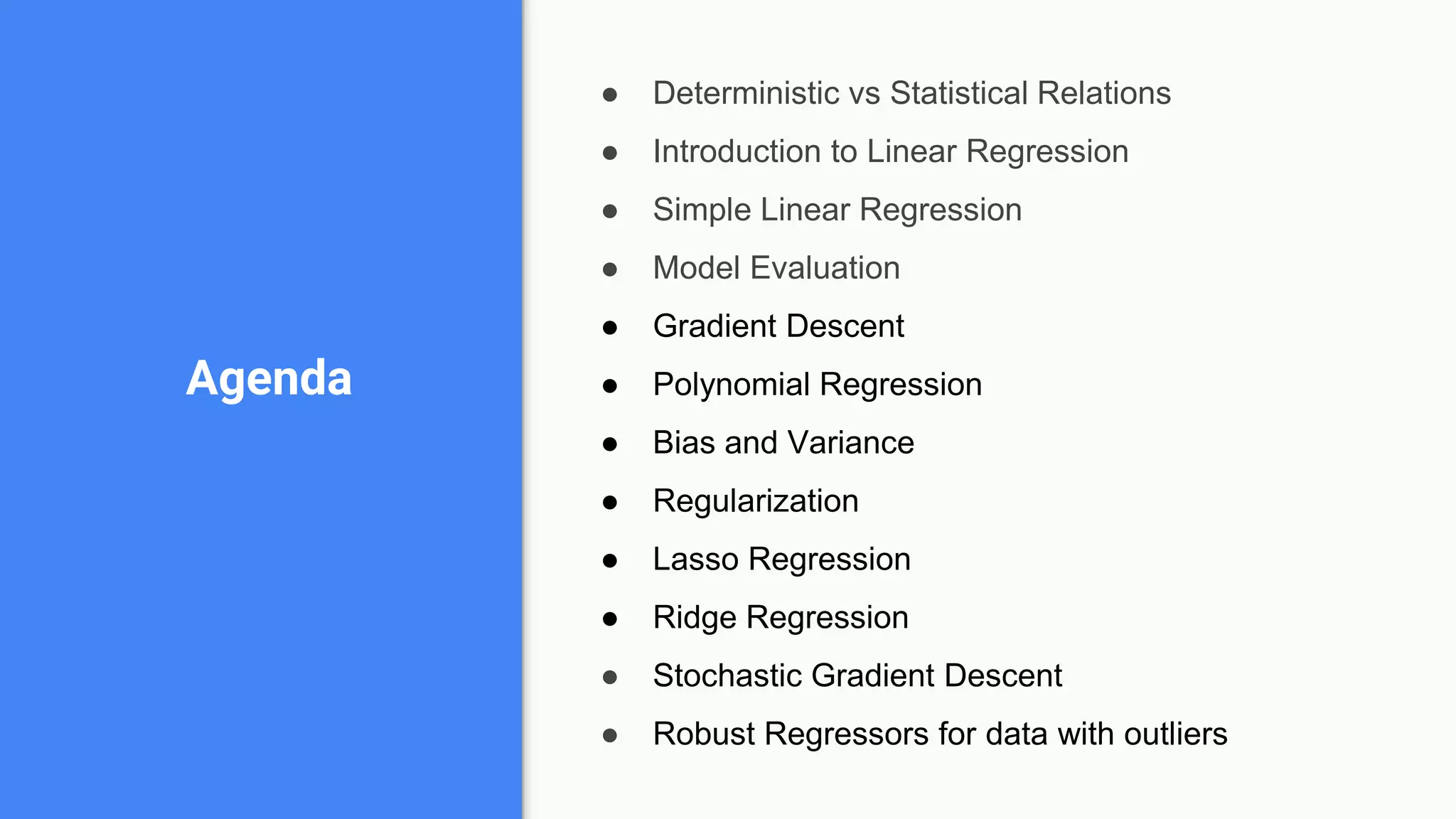

This document provides an overview of linear regression techniques. It begins with introducing deterministic vs statistical relationships and simple linear regression. It then covers model evaluation, gradient descent, and polynomial regression. The document discusses bias-variance tradeoff and various regularization techniques like lasso, ridge regression and stochastic gradient descent. It concludes with discussing robust regressors that are robust to outliers in the data.
Covers the basic concepts of Linear Regression, setting goals for becoming a Data Scientist, and agenda of topics including model evaluation.
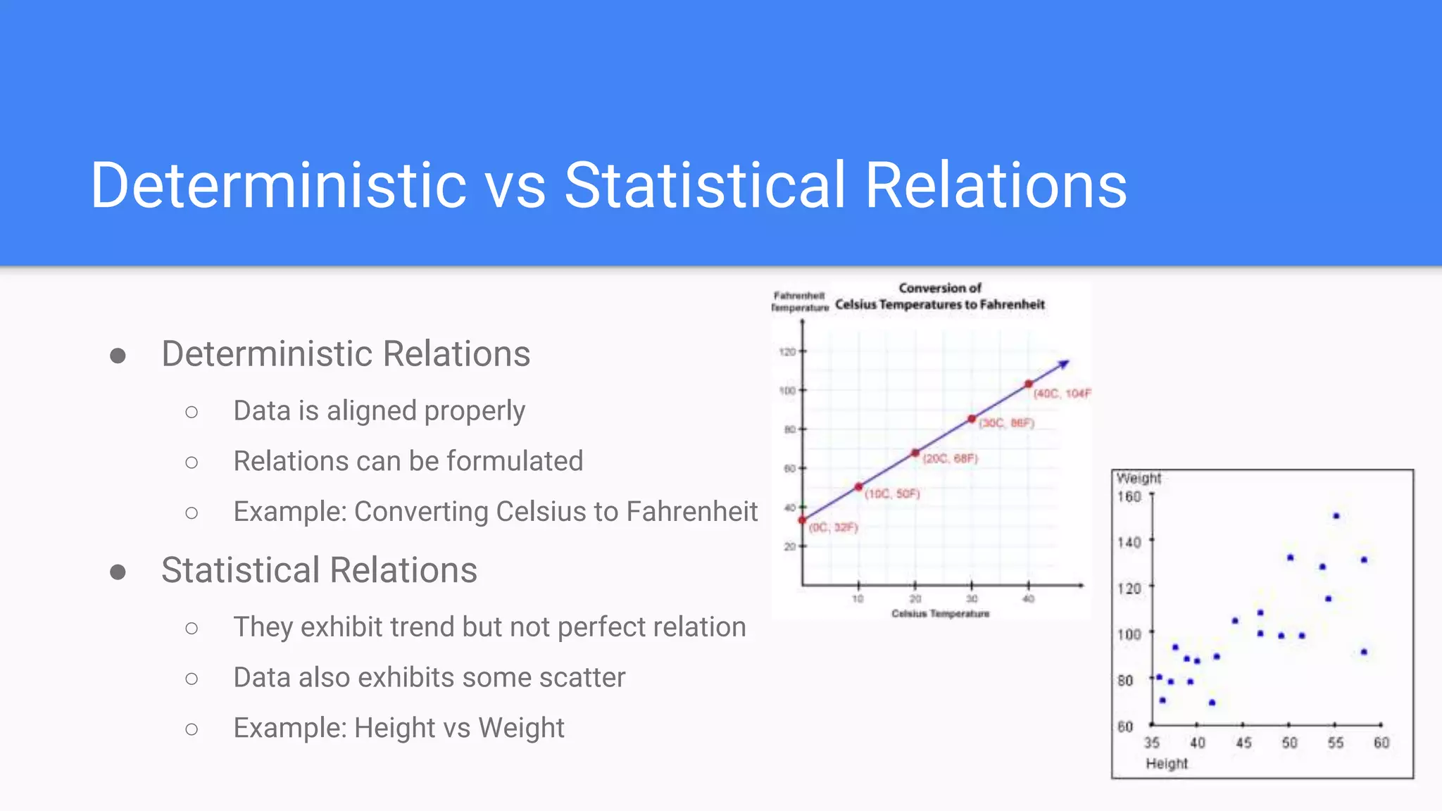
Explains deterministic and statistical relations with examples like Celsius to Fahrenheit and height vs weight.
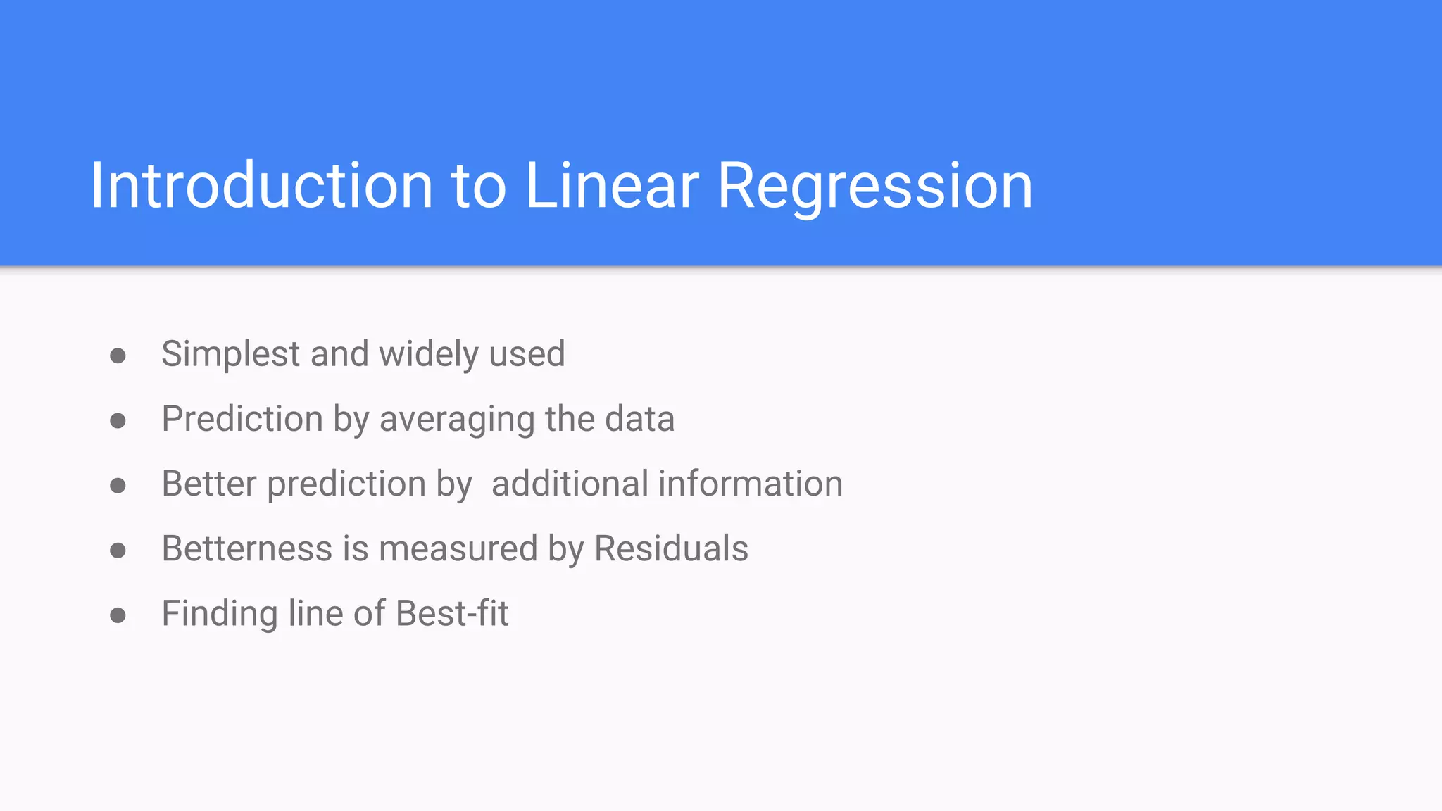
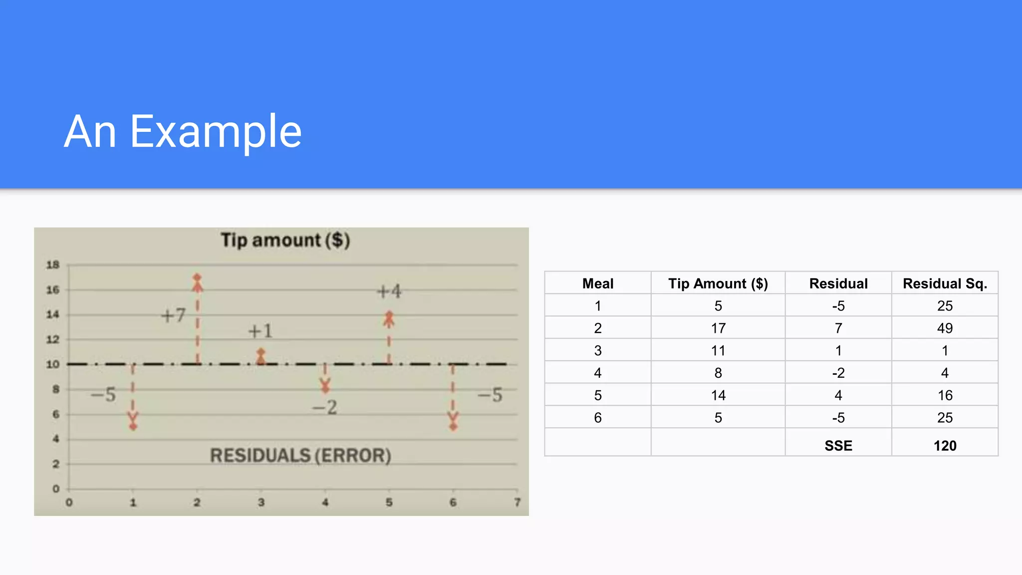
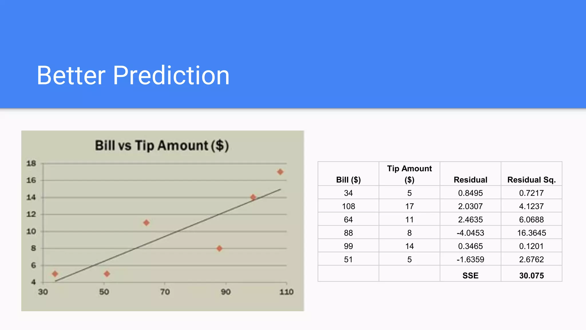
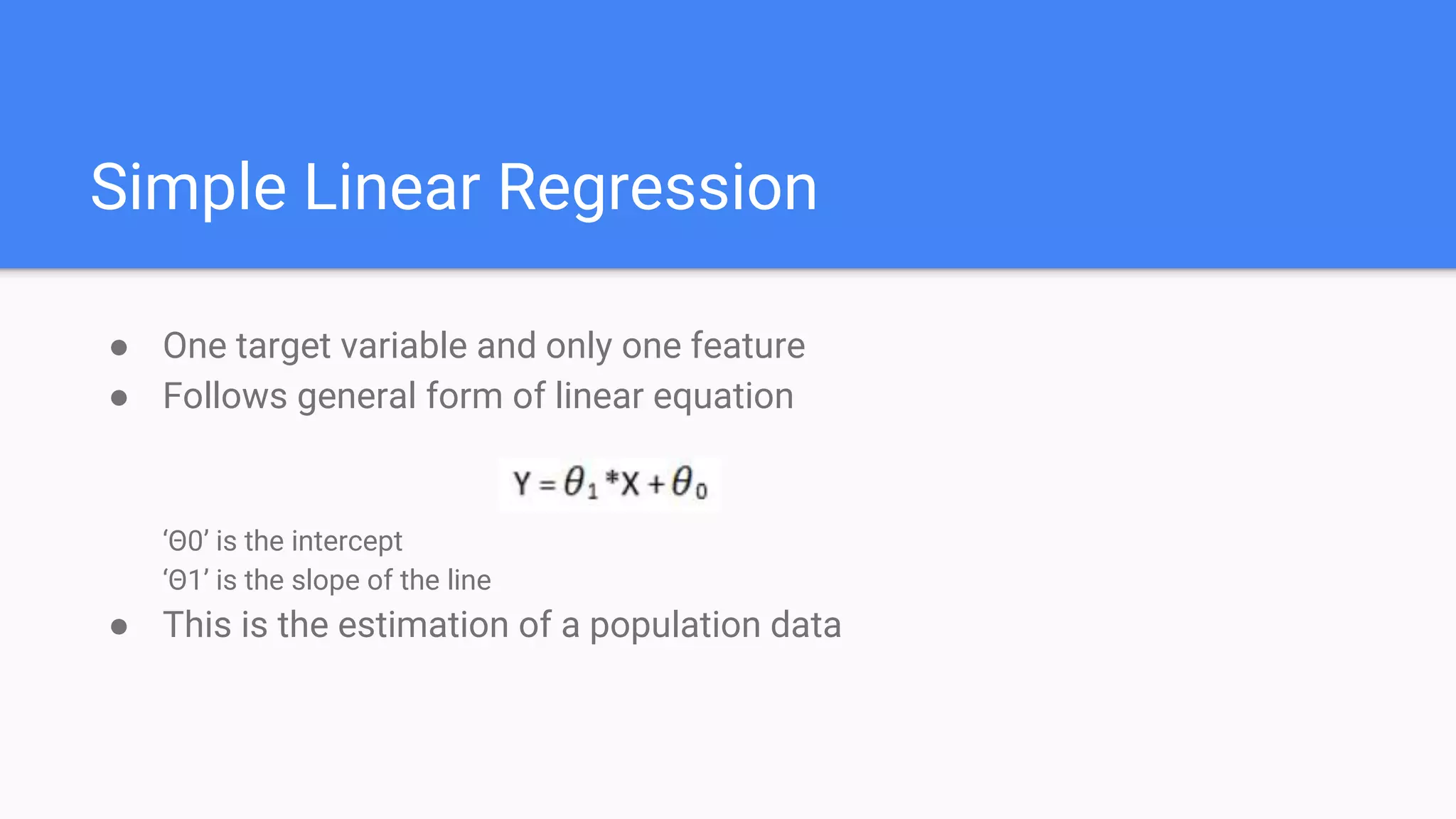
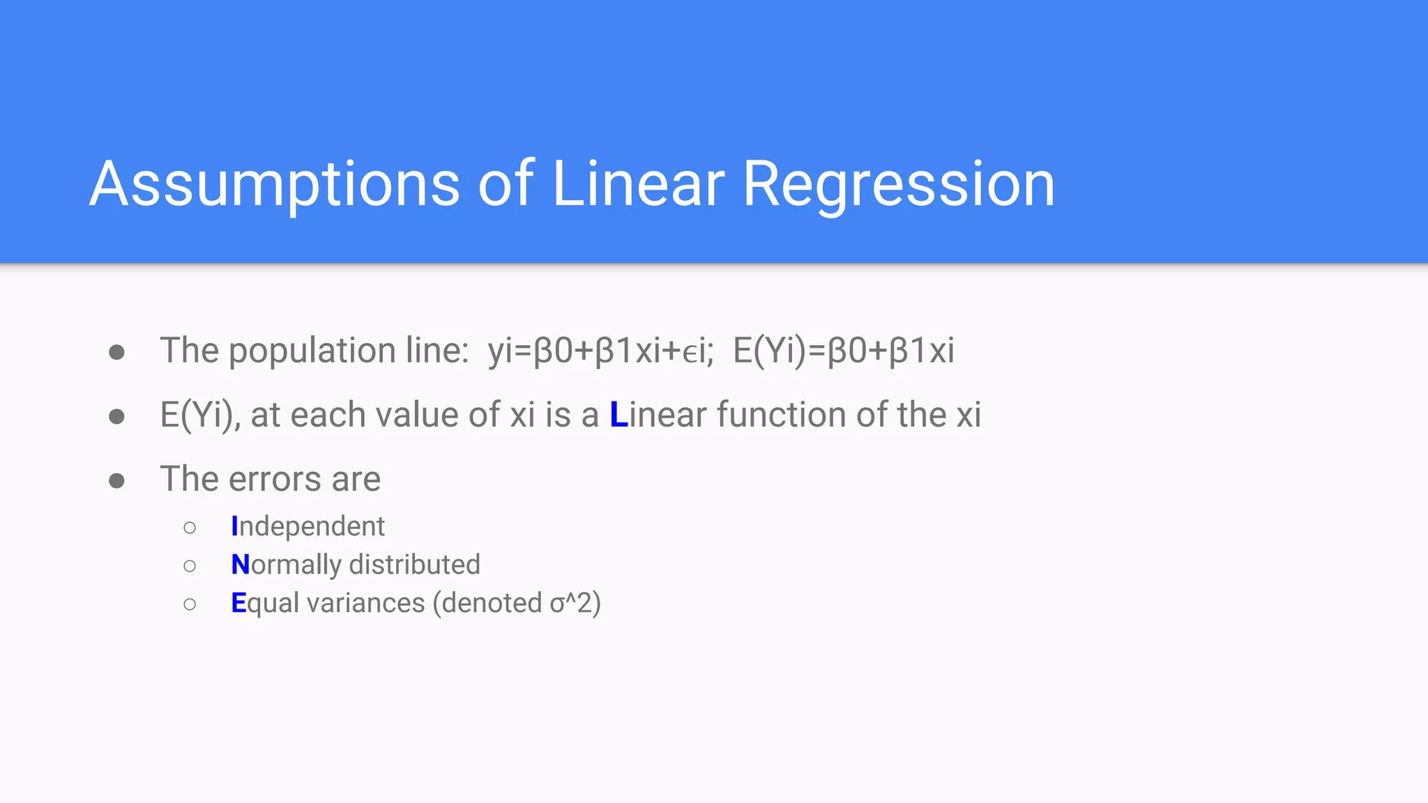
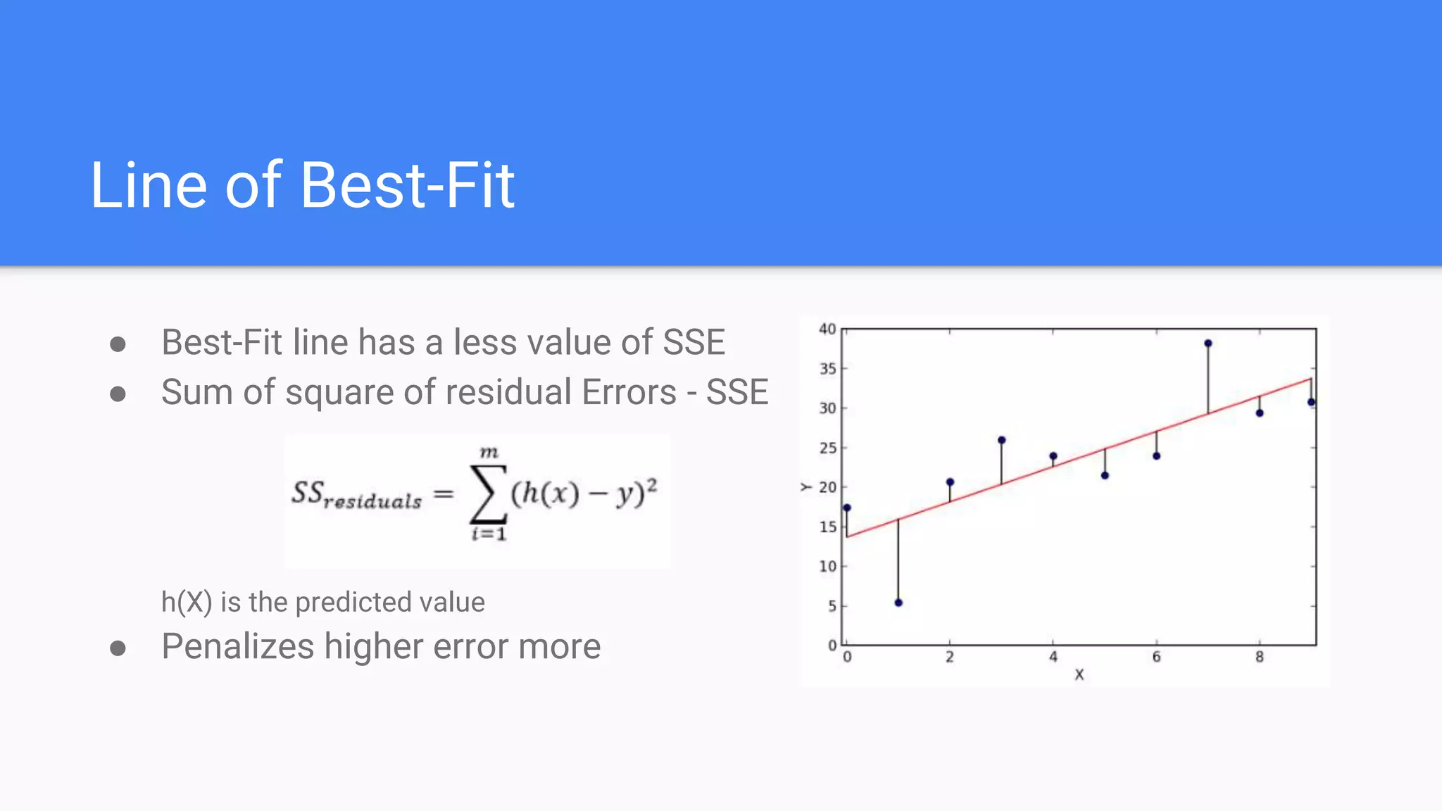
Discusses the fundamentals of linear regression including prediction, line of best-fit, residuals, and assumptions.
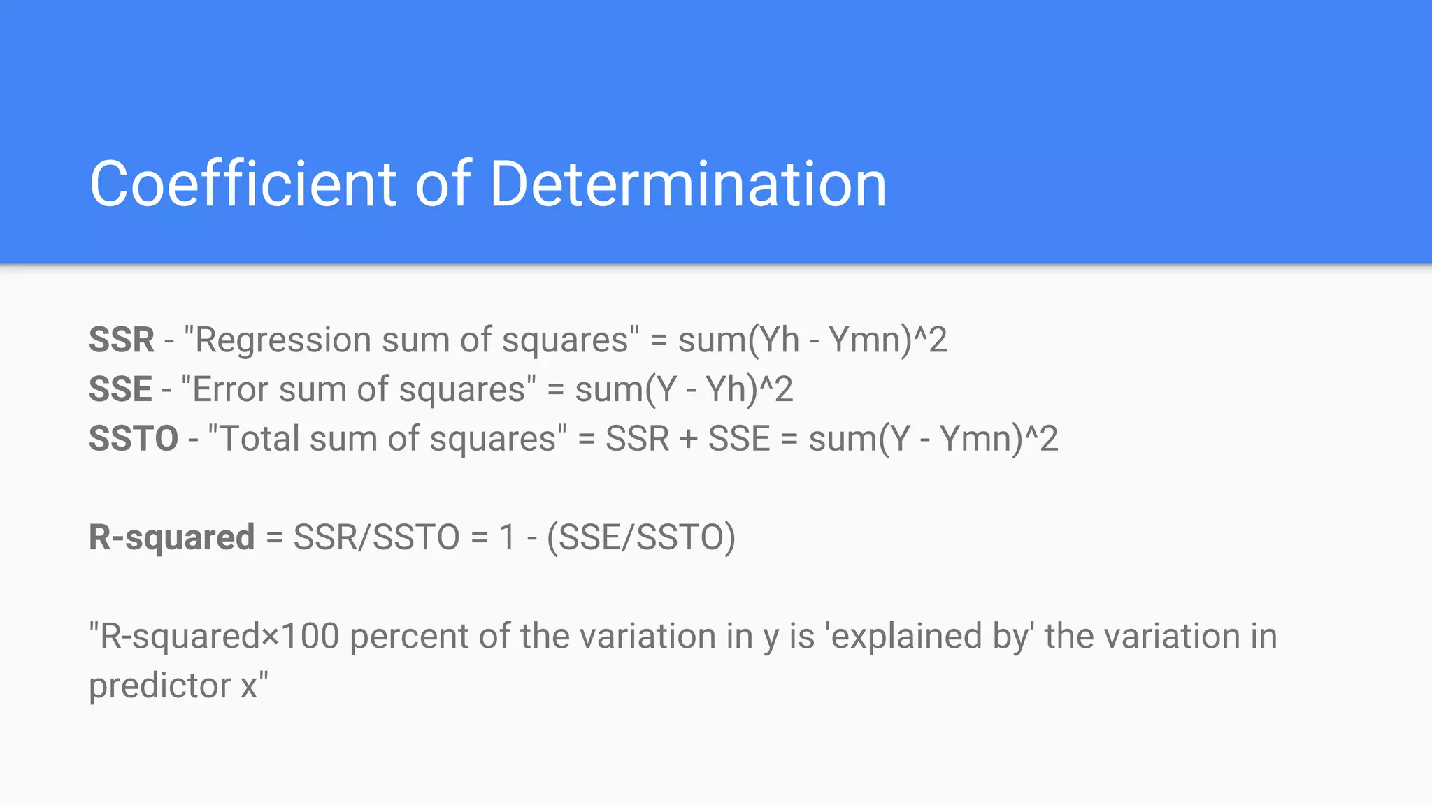
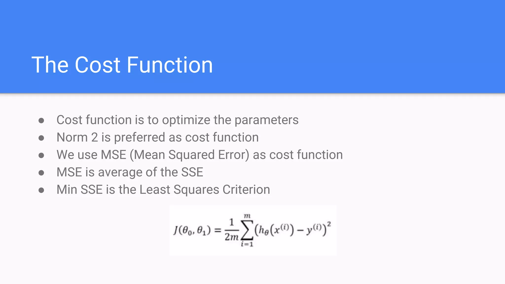
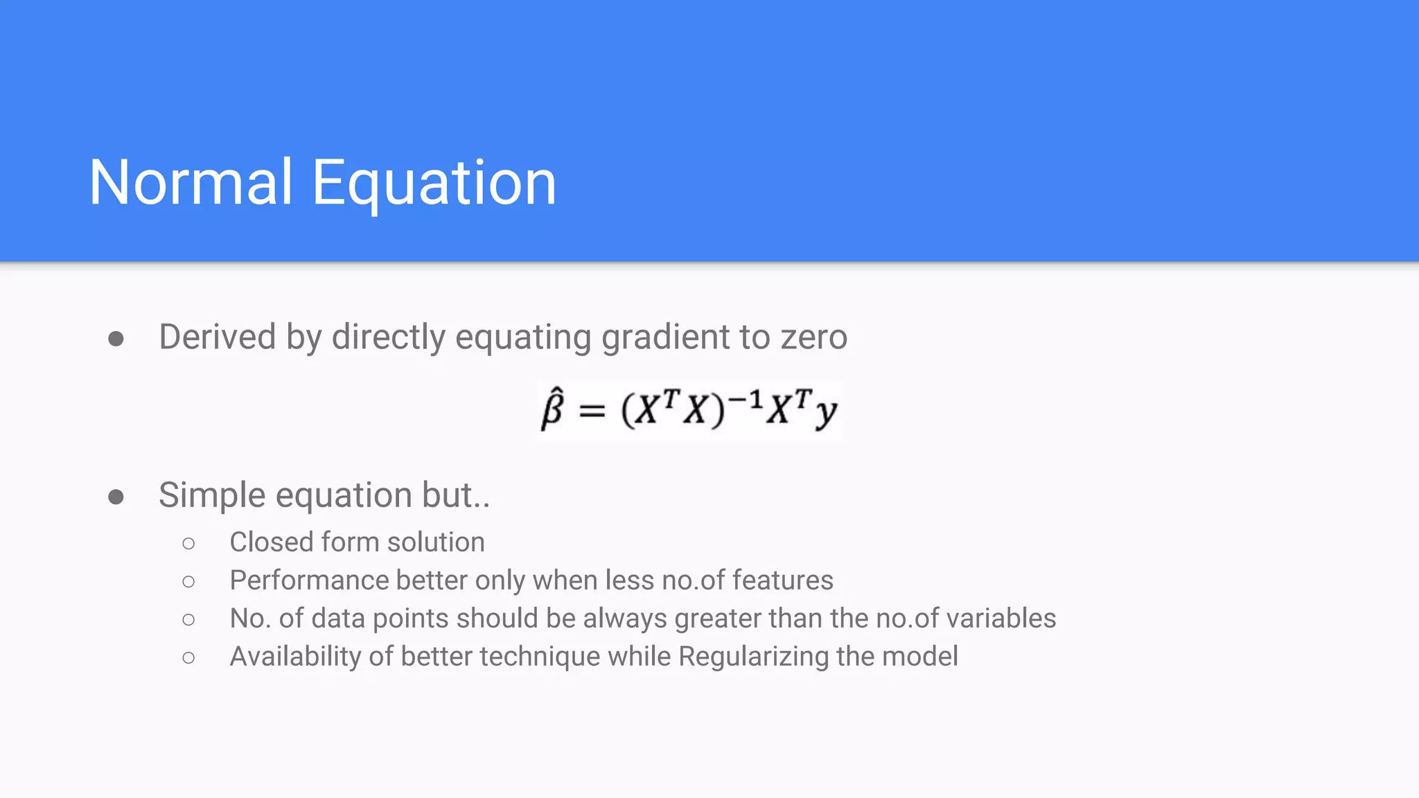
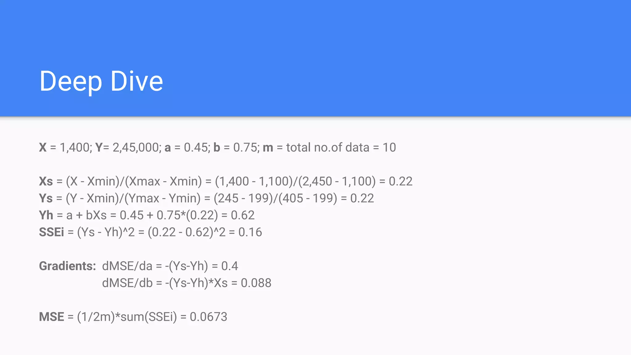
Introduces the coefficients of determination, SSE, and the cost function using Mean Squared Error for optimization.
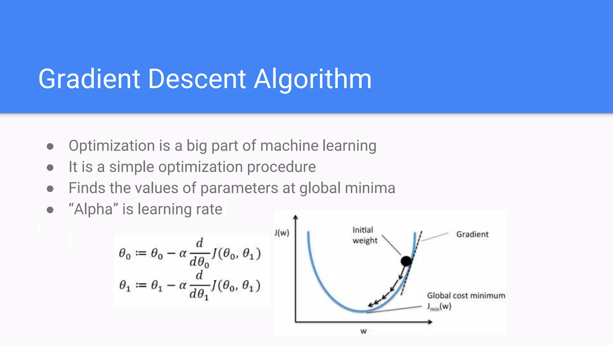
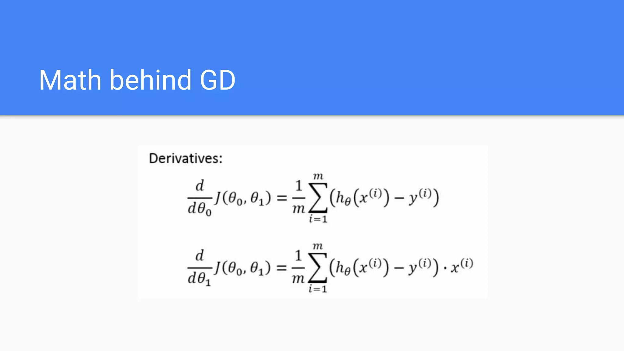
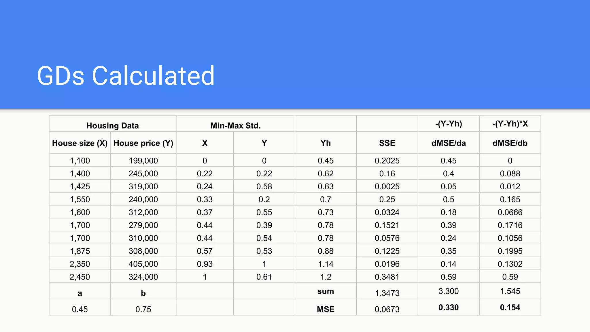
Details the gradient descent algorithm, its calculations, and how it helps in optimizing linear regression parameters.
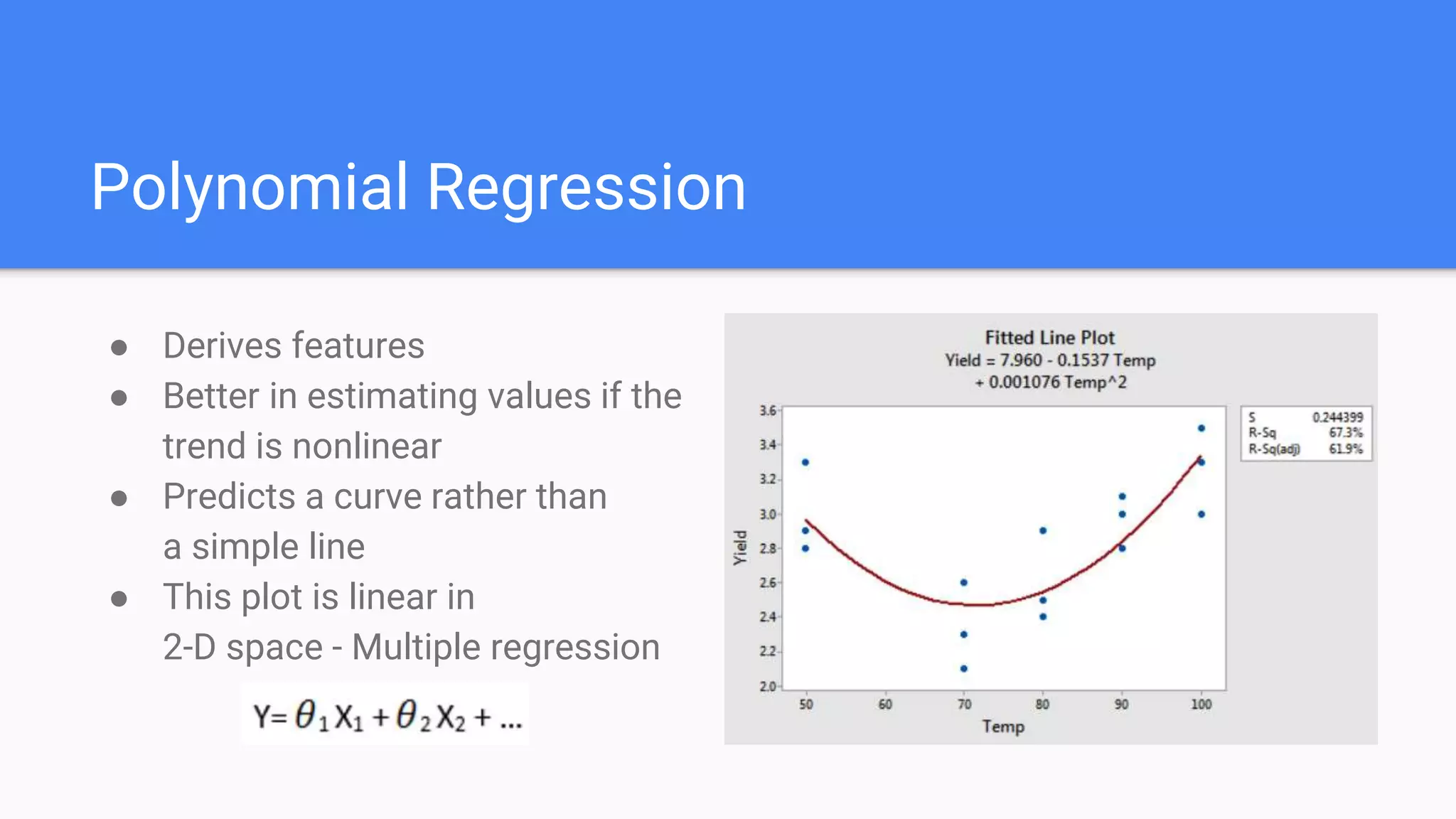
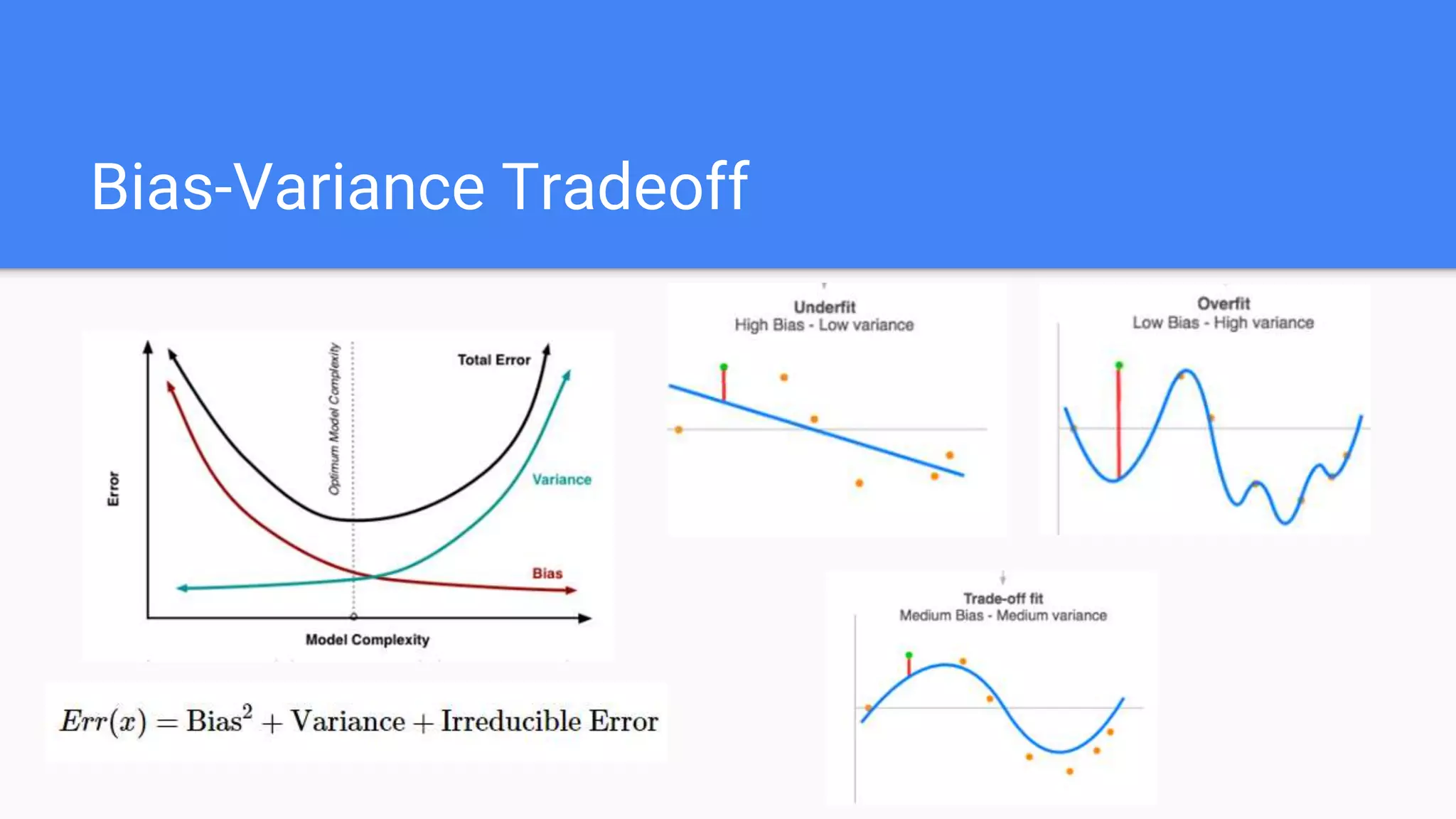
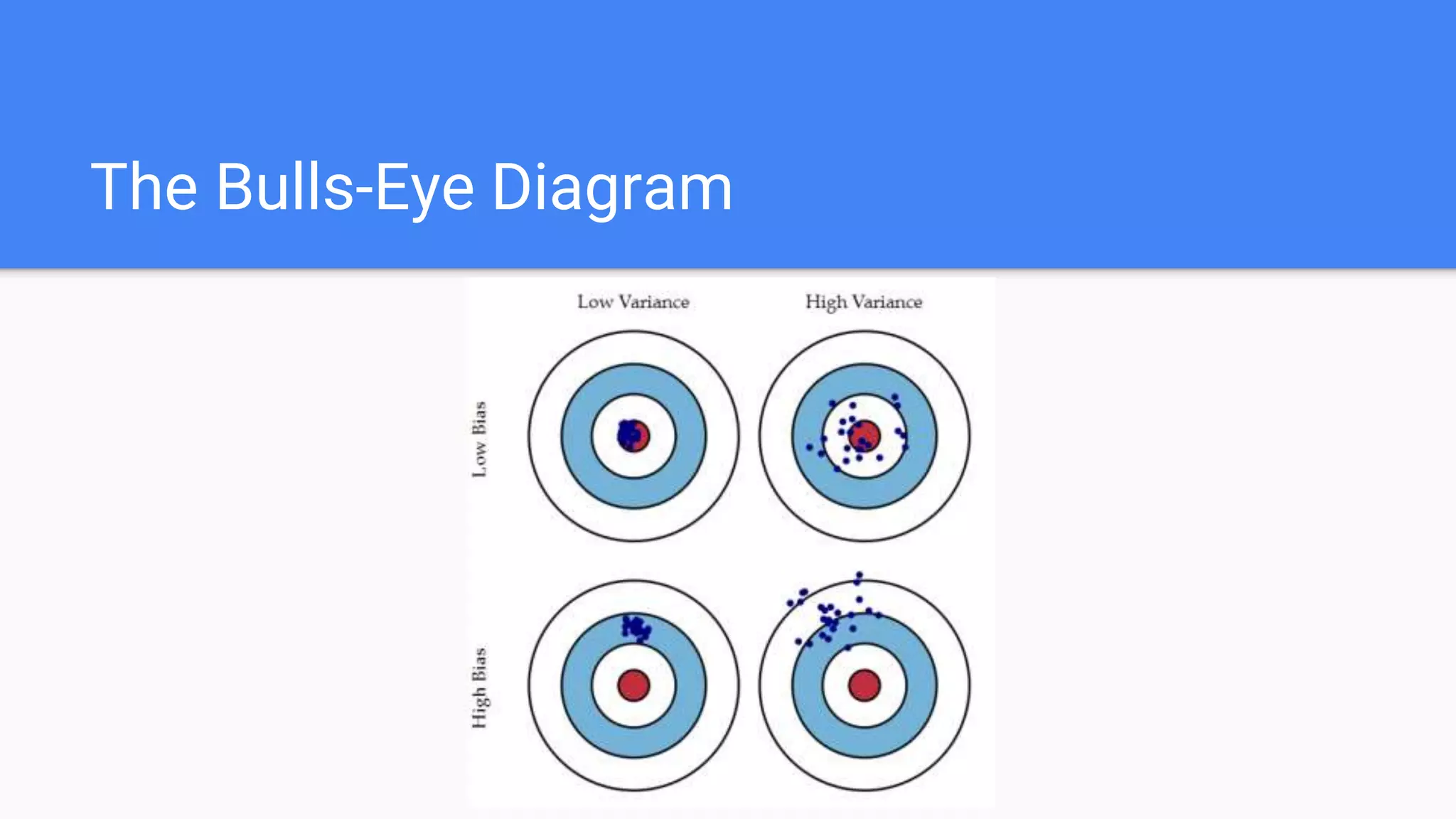
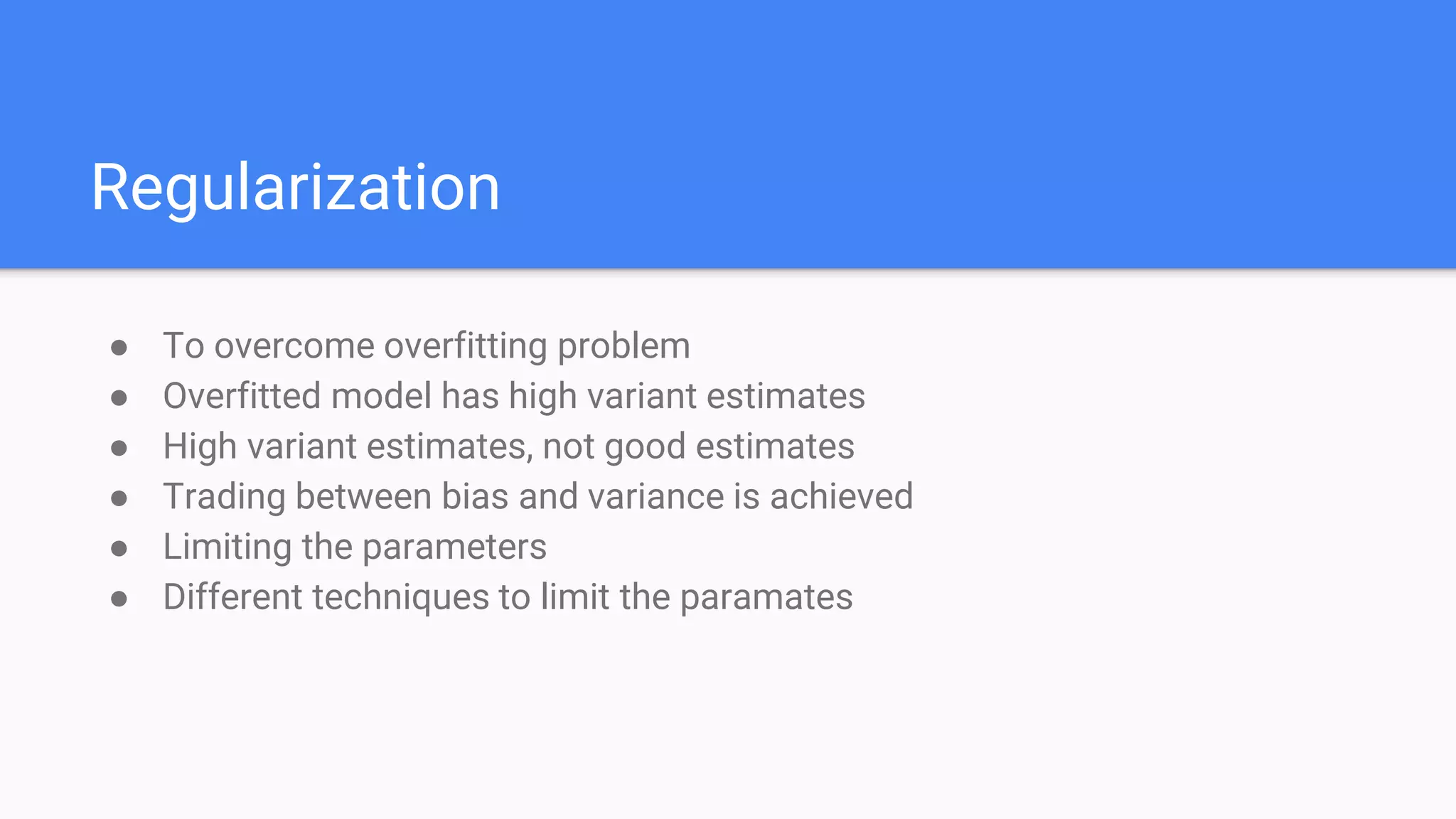
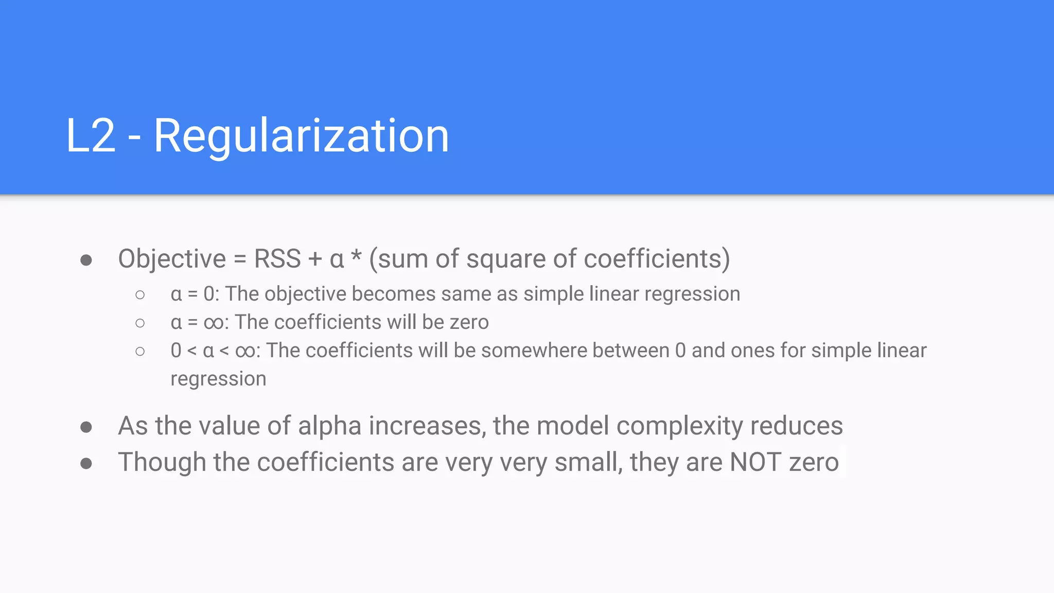
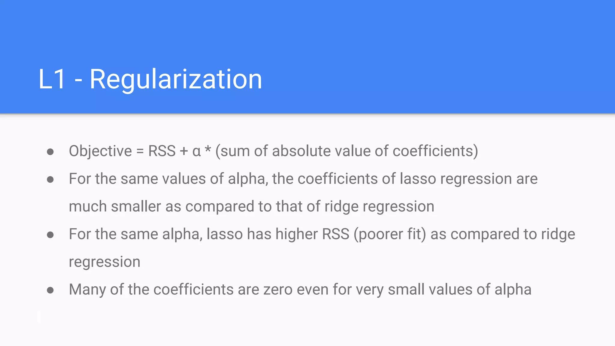
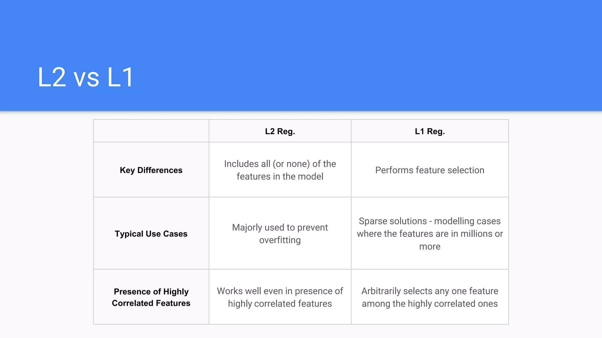
Explains polynomial regression, bias-variance tradeoff, regularization (L1 & L2), and differences between the two.
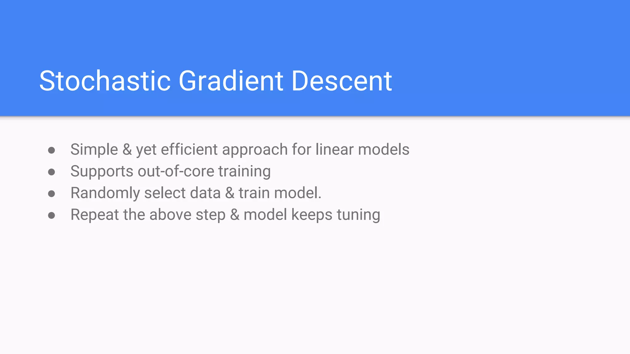
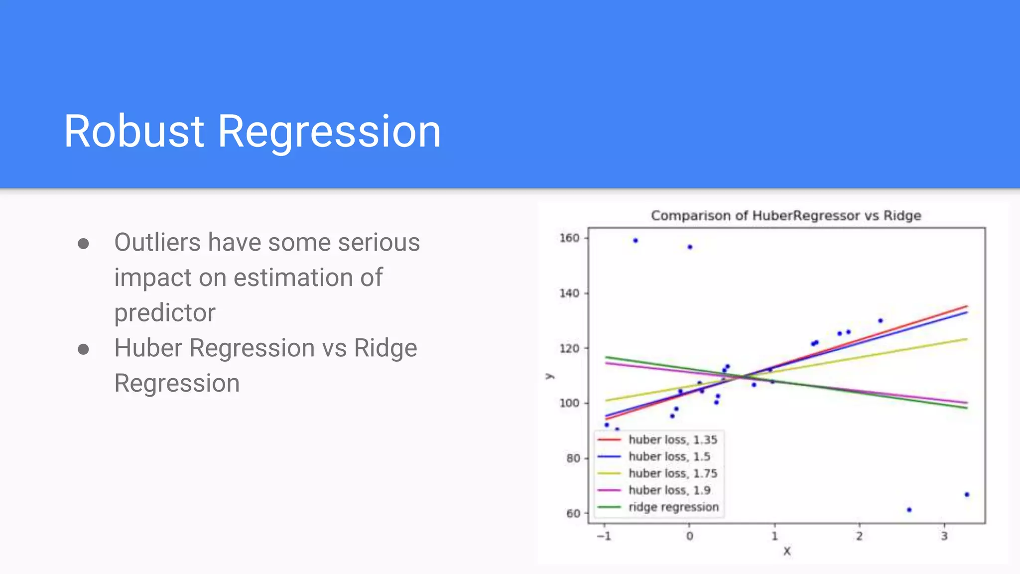
Highlights Stochastic Gradient Descent and the importance of Robust Regression to handle outliers effectively.


![[Webinar] Following the Agile Footprint - zekeLabs](https://cdn.slidesharecdn.com/ss_thumbnails/followingtheagilefootprint-webinar-200130092825-thumbnail.jpg?width=640&height=640&fit=bounds)


![Vibe Coding vs. Spec-Driven Development [Free Meetup]](https://cdn.slidesharecdn.com/ss_thumbnails/vibecodingvsspecdrivendevelopment-251209105622-43f455e7-thumbnail.jpg?width=640&height=640&fit=bounds)


