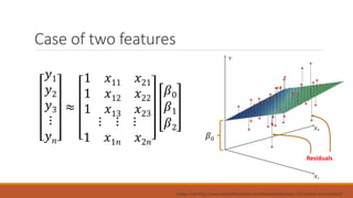
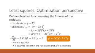
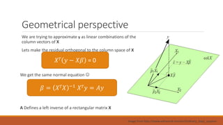
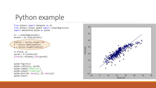
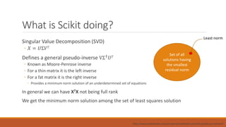
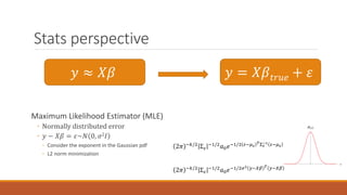
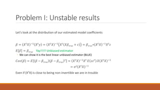
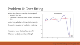
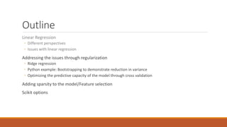
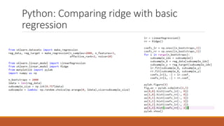
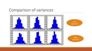
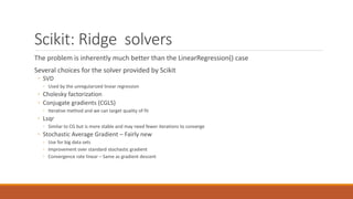
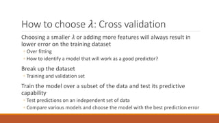
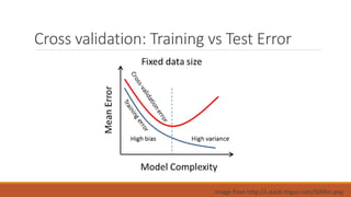
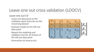
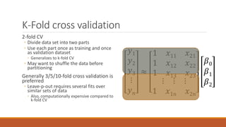
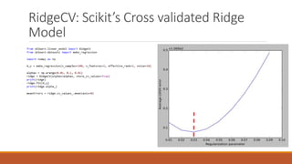
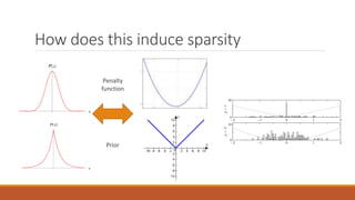
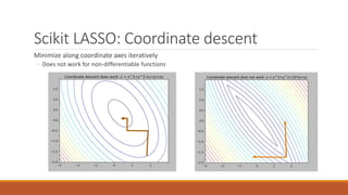
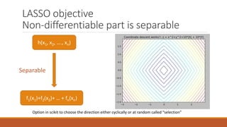
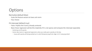
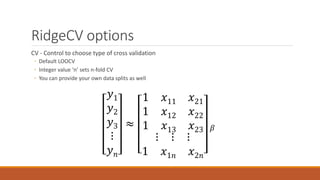
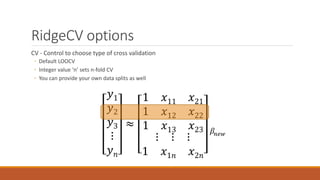
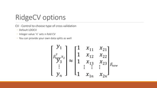
Linear Regression
ACM SIGKDD ADVANCED ML SERIES
ASHISH SRIVASTAVA (ANSRIVAS@GMAIL.COM)
Outline
Linear Regression
◦ Different perspectives
◦ Issues with linear regression
Addressing the issues through regularization
Adding sparsity to the model/Feature selection
Scikit options
Regression
Modeling a quantity as a simple function of features
◦ The predicted quantity should be well approximated as continuous
◦ Prices, lifespan, physical measurements
◦ As opposed to classification where we seek to predict discrete classes
Python example for today: Boston house prices
◦ The model is a linear function of the features
◦ House_price = a*age + b*House_size + ….
◦ Create nonlinear features to capture non-linearities
◦ House_size2 = house_size*house_size
◦ House_price = a*age + b*House_size + c*House_size2 + …..
Case of two features
Image from http://www.pieceofshijiabian.com/dataandstats/stats-216-lecture-notes/week3/
𝑦1
𝑦2
𝑦3
⋮
𝑦 𝑛
≈
1 𝑥11 𝑥21
1 𝑥12 𝑥22
1 𝑥13 𝑥23
⋮ ⋮ ⋮
1 𝑥1𝑛 𝑥2𝑛
𝛽0
𝛽1
𝛽2
𝛽0
Residuals
Linear Regression
 Model a quantity as a linear function of some known features
 𝑦 is the quantity to be modeled
 𝑋 are the sample points with each row being one data point
Columns are feature vectors
 Goal: Estimate the model coefficients or 𝛽
𝑦 ≈ 𝑋𝛽
Least squares: Optimization perspective
Define objective function using the 2-norm of the
residuals
◦ 𝑟𝑒𝑠𝑖𝑑𝑢𝑎𝑙𝑠 = 𝑦 − 𝑋𝛽
◦ Minimize: 𝑓 𝑜𝑏𝑗 = 𝑦 − 𝑋𝛽 2
2
= 𝑦 − 𝑋𝛽 𝑇 𝑦 − 𝑋𝛽
= 𝛽 𝑇 𝑋 𝑇 𝑋𝛽 − 2𝑦 𝑇 𝑋𝛽 + 𝑦 𝑇 𝑦
◦
𝜕𝑓 𝑜𝑏𝑗
𝜕𝛽
= 2𝑋 𝑇 𝑋𝛽 − 2𝑋 𝑇 𝑦 = 0
◦ Normal equation
◦ X is assumed to be thin and full rank so that 𝑋 𝑇 𝑋 is invertible
𝛽 = 𝑋 𝑇 𝑋 −1 𝑋 𝑇 𝑦
Geometrical perspective
We are trying to approximate y as linear combinations of the
column vectors of X
Lets make the residual orthogonal to the column space of X
We get the same normal equation 
A Defines a left inverse of a rectangular matrix X
𝑋 𝑇 𝑦 − 𝑋𝛽 = 0
𝛽 = 𝑋 𝑇 𝑋 −1 𝑋 𝑇 𝑦 = 𝐴𝑦
Image from http://www.wikiwand.com/en/Ordinary_least_squares
Python Example
Python example
What is Scikit doing?
http://www.mathworks.com/company/newsletters/articles/professor-svd.html
Singular Value Decomposition (SVD)
◦ 𝑋 = 𝑈Σ𝑉 𝑇
Defines a general pseudo-inverse VΣ† 𝑈 𝑇
◦ Known as Moore-Penrose inverse
◦ For a thin matrix it is the left inverse
◦ For a fat matrix it is the right inverse
◦ Provides a minimum norm solution of an underdetermined set of equations
In general we can have XTX not being full rank
We get the minimum norm solution among the set of least squares solution
Set of all
solutions having
the smallest
residual norm
Least norm
Stats perspective
Maximum Likelihood Estimator (MLE)
◦ Normally distributed error
◦ 𝑦 − 𝑋𝛽 = 𝜀~𝑁 0, 𝜎2 𝐼
◦ Consider the exponent in the Gaussian pdf
◦ L2 norm minimization
𝑦 ≈ 𝑋𝛽 𝑦 = 𝑋𝛽𝑡𝑟𝑢𝑒 + 𝜀
2𝜋 −𝑘/2
Σ 𝜀
−1/2
𝑎0 𝑒−1/2 𝜀−𝜇 𝜀
𝑇Σ 𝜀
−1 𝜀−𝜇 𝜀
2𝜋 −𝑘/2 Σ 𝜀
−1/2 𝑎0 𝑒−1/2𝜎2 𝑦−𝑋𝛽 𝑇 𝑦−𝑋𝛽
Let’s look at the distribution of our estimated model coefficients
𝛽 = 𝑋 𝑇 𝑋 −1 𝑋 𝑇 𝑦 = 𝑋 𝑇 𝑋 −1 𝑋 𝑇 𝑋𝛽𝑡𝑟𝑢𝑒 + 𝜀 = 𝛽𝑡𝑟𝑢𝑒+ 𝑋 𝑇 𝑋 −1 𝑋 𝑇 𝜀
𝐸 𝛽 = 𝛽𝑡𝑟𝑢𝑒 Yay!!!!! Unbiased estimator
◦ We can show it is the best linear unbiased estimator (BLUE)
𝐶𝑜𝑣 𝛽 = 𝐸 𝛽 − 𝛽𝑡𝑟𝑢𝑒 𝛽 − 𝛽𝑡𝑟𝑢𝑒
𝑇 = 𝑋 𝑇 𝑋 −1
𝑋 𝑇 𝐸 𝜀𝜀 𝑇 𝑋 𝑋 𝑇 𝑋 −1
= 𝜎2 𝑋 𝑇 𝑋 −1
Even if (XTX) is close to being non-invertible we are in trouble
Problem I: Unstable results
Estimate parameter variance
Bootstrapping
Problem II: Over fitting
Model describes the training data very well
◦ Actually “too” well
◦ The model is adapting to any noise in the training
data
Model is very bad predicting at other points
Defeats the purpose of predictive modeling
How do we know that we have overfit?
What can we do to avoid overfitting?
Image from http://blog.rocapal.org/?p=423
Outline
Linear Regression
◦ Different perspectives
◦ Issues with linear regression
Addressing the issues through regularization
◦ Ridge regression
◦ Python example: Bootstrapping to demonstrate reduction in variance
◦ Optimizing the predictive capacity of the model through cross validation
Adding sparsity to the model/Feature selection
Scikit options
Minimize: ||𝑦 − 𝑋𝛽||2
2
Ridge Regression / Tikhonov regularization
A biased linear estimator to get better variance
◦ Least squares was BLUE so we cant hope to get better variance while staying unbiased
Gaussian MLE with a Gaussian prior on the model coefficients
𝑋 𝑇 𝑋 + 𝜆𝐼 𝛽= 𝑋 𝑇y
Minimize: ||𝑦 − 𝑋𝛽||2
2
+ λ||𝛽||2
2
Python example: Creating testcases
make_regression in scikit.datasets
◦ Several parameters to control the “type” of dataset we want
◦ Parameters:
◦ Size: n_samples and n_features
◦ Type: n_informative, effective_rank, tail_strength, noise
We want to test ridge regression with datasets with a low effective rank
◦ Highly correlated (or linearly dependent) features
Python: Comparing ridge with basic
regression
Comparison of variances
Linear
regression
Ridge
regression
Scikit: Ridge solvers
The problem is inherently much better than the LinearRegression() case
Several choices for the solver provided by Scikit
◦ SVD
◦ Used by the unregularized linear regression
◦ Cholesky factorization
◦ Conjugate gradients (CGLS)
◦ Iterative method and we can target quality of fit
◦ Lsqr
◦ Similar to CG but is more stable and may need fewer iterations to converge
◦ Stochastic Average Gradient – Fairly new
◦ Use for big data sets
◦ Improvement over standard stochastic gradient
◦ Convergence rate linear – Same as gradient descent
How to choose 𝜆: Cross validation
Choosing a smaller 𝜆 or adding more features will always result in
lower error on the training dataset
◦ Over fitting
◦ How to identify a model that will work as a good predictor?
Break up the dataset
◦ Training and validation set
Train the model over a subset of the data and test its predictive
capability
◦ Test predictions on an independent set of data
◦ Compare various models and choose the model with the best prediction error
Cross validation: Training vs Test Error
Image from http://i.stack.imgur.com/S0tRm.png
Leave one out cross validation (LOOCV)
Leave one out CV
◦ Leave one data point as the
validation point and train on the
remaining dataset
◦ Evaluate model on the left out
data point
◦ Repeat the modeling and
validation test for all choices of
the left out data point
◦ Generalizes to leave-p-out
𝑦1
𝑦2
𝑦3
⋮
𝑦 𝑛
≈
1 𝑥11 𝑥21
1 𝑥12 𝑥22
1 𝑥13 𝑥23
⋮ ⋮ ⋮
1 𝑥1𝑛 𝑥2𝑛
𝛽0
𝛽1
𝛽2
K-Fold cross validation
2-fold CV
◦ Divide data set into two parts
◦ Use each part once as training and once
as validation dataset
◦ Generalizes to k-fold CV
◦ May want to shuffle the data before
partitioning
Generally 3/5/10-fold cross validation is
preferred
◦ Leave-p-out requires several fits over
similar sets of data
◦ Also, computationally expensive compared to
k-fold CV
𝑦1
𝑦2
𝑦3
⋮
𝑦 𝑛
≈
1 𝑥11 𝑥21
1 𝑥12 𝑥22
1 𝑥13 𝑥23
⋮ ⋮ ⋮
1 𝑥1𝑛 𝑥2𝑛
𝛽0
𝛽1
𝛽2
RidgeCV: Scikit’s Cross validated Ridge
Model
Outline
Linear Regression
◦ Different perspectives
◦ Issues with linear regression
Addressing the issues through regularization
◦ Ridge regression
◦ Python example: Bootstrapping to demonstrate reduction in variance
◦ Optimizing the predictive capacity of the model through cross validation
Adding sparsity to the model/Feature selection
◦ LASSO
◦ Basis Pursuit Methods: Matching Pursuit and Least Angle regression
Scikit options
LASSO
The penalty term for coefficient sizes is now the l1 norm
Gaussian MLE with a laplacian prior distribution on the parameters
Can result in many feature coefficients being zero/sparse solution
◦ Can be used to select a subset of features – Feature selection
Minimize: ||𝑦 − 𝑋𝛽||2
2
Minimize: ||𝑦 − 𝑋𝛽||2
2
+ λ||𝛽||1
How does this induce sparsity
Penalty
function
Prior
Scikit LASSO: Coordinate descent
Minimize along coordinate axes iteratively
◦ Does not work for non-differentiable functions
LASSO objective
Non-differentiable part is separable
h(x1, x2, …., xn)
f1(x1)+f2(x2)+ … + fn(xn)
Separable
Option in scikit to choose the direction either cyclically or at random called “selection”
Matching Pursuit (MP)
Select feature most correlated to the residual
f1
f2
Orthogonal Matching Pursuit (OMP)
Keep residual orthogonal to the set of selected features
(O)MP methods are greedy
◦ Correlated features are ignored and will not be considered again
f1
f2
LARS (Least Angle regression)
Move along most correlated feature until another feature becomes equally correlated
f1
f2
Outline
Linear Regression
◦ Different perspectives
◦ Issues with linear regression
Addressing the issues through regularization
◦ Ridge regression
◦ Python example: Bootstrapping to demonstrate reduction in variance
◦ Optimizing the predictive capacity of the model through cross validation
Adding sparsity to the model/Feature selection
◦ LASSO
◦ Basis Pursuit Methods: Matching Pursuit and Least Angle regression
Scikit options
Options
Normalize (default false)
◦ Scale the feature vectors to have unit norm
◦ Your choice
Fit intercept (default true)
◦ False: Implies the X and y already centered
◦ Basic linear regression will do this implicitly if X is not sparse and compute the intercept separately
◦ Centering can kill sparsity
◦ Center data matrix in regularized regressions unless you really want a penalty on the bias
◦ Issues with sparsity still being worked out in scikit (Temporary bug fix for ridge in 0.17 using sag solver)
RidgeCV options
CV - Control to choose type of cross validation
◦ Default LOOCV
◦ Integer value ‘n’ sets n-fold CV
◦ You can provide your own data splits as well
𝑦1
𝑦2
𝑦3
⋮
𝑦 𝑛
≈
1 𝑥11 𝑥21
1 𝑥12 𝑥22
1 𝑥13 𝑥23
⋮ ⋮ ⋮
1 𝑥1𝑛 𝑥2𝑛
𝛽
RidgeCV options
CV - Control to choose type of cross validation
◦ Default LOOCV
◦ Integer value ‘n’ sets n-fold CV
◦ You can provide your own data splits as well
𝑦1
𝑦2
𝑦3
⋮
𝑦 𝑛
≈
1 𝑥11 𝑥21
1 𝑥12 𝑥22
1 𝑥13 𝑥23
⋮ ⋮ ⋮
1 𝑥1𝑛 𝑥2𝑛
𝛽𝑛𝑒𝑤
RidgeCV options
CV - Control to choose type of cross validation
◦ Default LOOCV
◦ Integer value ‘n’ sets n-fold CV
◦ You can provide your own data splits as well
𝑦1
𝛽𝑛𝑒𝑤
𝑇
𝑥2
𝑦3
⋮
𝑦 𝑛
≈
1 𝑥11 𝑥21
1 𝑥12 𝑥22
1 𝑥13 𝑥23
⋮ ⋮ ⋮
1 𝑥1𝑛 𝑥2𝑛
𝛽𝑛𝑒𝑤
Lasso(CV)/Lars(CV) options
Positive
◦ Force coefficients to be positive
Other controls for iterations
◦ Number of iterations (Lasso) / Number of non-zeros (Lars)
◦ Tolerance to stop iterations (Lasso)
Summary
Linear Models
◦ Linear regression
◦ Ridge – L2 penalty
◦ Lasso – L1 penalty results in sparsity
◦ LARS – Select a sparse set of features iteratively
Use Cross Validation (CV) to choose your models – Leverage scikit
◦ RidgeCV, LarsCV, LassoCV
Not discussed – Explore scikit
◦ Combing Ridge and Lasso: Elastic Nets
◦ Random Sample Consensus (RANSAC)
◦ Fitting linear models where data has several outliers
◦ lassoLars, lars_path
References
All code examples are taken form “Scikit-Learn Cookbook” by Trent Hauck with some slight
modifications
LSQR -> C. C. Paige and M. A. Saunders, LSQR: An algorithm for sparse linear equations and
sparse least squares. 1982.
Ridge SAG -> Mark Schmidt, Nicolas Le Roux, Francis Bach: Minimizing Finite Sums with the
Stochastic Average Gradient. 2013.
Ridge CV LOOCV -> Rifkin, Lippert: Notes on Regularized Least Squares, MIT Technical Report.
2007.
BP Methods1 -> Bradley Efron, Trevor Hastie, Iain Johnstone, and Robert Tibshirani: Least Angle
Regression. 2004.
BP Methods2 -> Hameed: Comparative Analysis of Orthogonal Matching Pursuit and Least Angle
Regression, MSU MS Thesis. 2012.
BACKUP
Python example
Stochastic Gradient Descent
When we have an immense number of samples or features SGD can come in handy
Randomly select a sample point and use that to evaluate a gradient direction in which to move
the parameters
◦ Repeat the procedure until a “tolerance” is achieved
Normalizing the data is important
Recursive least squares
Suppose a scenario in which we sequentially obtain a sample point and measurement and we
would like to continually update our least squares estimate
◦ “Incremental” least squares estimate
◦ Rank one update of the matrix XTX
Utilize the matrix inversion lemma
Similar idea used in RidgeCV LOOCV

Linear regression

  • 1.
    Linear Regression ACM SIGKDDADVANCED ML SERIES ASHISH SRIVASTAVA (ANSRIVAS@GMAIL.COM)
  • 2.
    Outline Linear Regression ◦ Differentperspectives ◦ Issues with linear regression Addressing the issues through regularization Adding sparsity to the model/Feature selection Scikit options
  • 3.
    Regression Modeling a quantityas a simple function of features ◦ The predicted quantity should be well approximated as continuous ◦ Prices, lifespan, physical measurements ◦ As opposed to classification where we seek to predict discrete classes Python example for today: Boston house prices ◦ The model is a linear function of the features ◦ House_price = a*age + b*House_size + …. ◦ Create nonlinear features to capture non-linearities ◦ House_size2 = house_size*house_size ◦ House_price = a*age + b*House_size + c*House_size2 + …..
  • 4.
    Case of twofeatures Image from http://www.pieceofshijiabian.com/dataandstats/stats-216-lecture-notes/week3/ 𝑦1 𝑦2 𝑦3 ⋮ 𝑦 𝑛 ≈ 1 𝑥11 𝑥21 1 𝑥12 𝑥22 1 𝑥13 𝑥23 ⋮ ⋮ ⋮ 1 𝑥1𝑛 𝑥2𝑛 𝛽0 𝛽1 𝛽2 𝛽0 Residuals
  • 5.
    Linear Regression  Modela quantity as a linear function of some known features  𝑦 is the quantity to be modeled  𝑋 are the sample points with each row being one data point Columns are feature vectors  Goal: Estimate the model coefficients or 𝛽 𝑦 ≈ 𝑋𝛽
  • 6.
    Least squares: Optimizationperspective Define objective function using the 2-norm of the residuals ◦ 𝑟𝑒𝑠𝑖𝑑𝑢𝑎𝑙𝑠 = 𝑦 − 𝑋𝛽 ◦ Minimize: 𝑓 𝑜𝑏𝑗 = 𝑦 − 𝑋𝛽 2 2 = 𝑦 − 𝑋𝛽 𝑇 𝑦 − 𝑋𝛽 = 𝛽 𝑇 𝑋 𝑇 𝑋𝛽 − 2𝑦 𝑇 𝑋𝛽 + 𝑦 𝑇 𝑦 ◦ 𝜕𝑓 𝑜𝑏𝑗 𝜕𝛽 = 2𝑋 𝑇 𝑋𝛽 − 2𝑋 𝑇 𝑦 = 0 ◦ Normal equation ◦ X is assumed to be thin and full rank so that 𝑋 𝑇 𝑋 is invertible 𝛽 = 𝑋 𝑇 𝑋 −1 𝑋 𝑇 𝑦
  • 7.
    Geometrical perspective We aretrying to approximate y as linear combinations of the column vectors of X Lets make the residual orthogonal to the column space of X We get the same normal equation  A Defines a left inverse of a rectangular matrix X 𝑋 𝑇 𝑦 − 𝑋𝛽 = 0 𝛽 = 𝑋 𝑇 𝑋 −1 𝑋 𝑇 𝑦 = 𝐴𝑦 Image from http://www.wikiwand.com/en/Ordinary_least_squares
  • 8.
  • 9.
  • 10.
    What is Scikitdoing? http://www.mathworks.com/company/newsletters/articles/professor-svd.html Singular Value Decomposition (SVD) ◦ 𝑋 = 𝑈Σ𝑉 𝑇 Defines a general pseudo-inverse VΣ† 𝑈 𝑇 ◦ Known as Moore-Penrose inverse ◦ For a thin matrix it is the left inverse ◦ For a fat matrix it is the right inverse ◦ Provides a minimum norm solution of an underdetermined set of equations In general we can have XTX not being full rank We get the minimum norm solution among the set of least squares solution Set of all solutions having the smallest residual norm Least norm
  • 11.
    Stats perspective Maximum LikelihoodEstimator (MLE) ◦ Normally distributed error ◦ 𝑦 − 𝑋𝛽 = 𝜀~𝑁 0, 𝜎2 𝐼 ◦ Consider the exponent in the Gaussian pdf ◦ L2 norm minimization 𝑦 ≈ 𝑋𝛽 𝑦 = 𝑋𝛽𝑡𝑟𝑢𝑒 + 𝜀 2𝜋 −𝑘/2 Σ 𝜀 −1/2 𝑎0 𝑒−1/2 𝜀−𝜇 𝜀 𝑇Σ 𝜀 −1 𝜀−𝜇 𝜀 2𝜋 −𝑘/2 Σ 𝜀 −1/2 𝑎0 𝑒−1/2𝜎2 𝑦−𝑋𝛽 𝑇 𝑦−𝑋𝛽
  • 12.
    Let’s look atthe distribution of our estimated model coefficients 𝛽 = 𝑋 𝑇 𝑋 −1 𝑋 𝑇 𝑦 = 𝑋 𝑇 𝑋 −1 𝑋 𝑇 𝑋𝛽𝑡𝑟𝑢𝑒 + 𝜀 = 𝛽𝑡𝑟𝑢𝑒+ 𝑋 𝑇 𝑋 −1 𝑋 𝑇 𝜀 𝐸 𝛽 = 𝛽𝑡𝑟𝑢𝑒 Yay!!!!! Unbiased estimator ◦ We can show it is the best linear unbiased estimator (BLUE) 𝐶𝑜𝑣 𝛽 = 𝐸 𝛽 − 𝛽𝑡𝑟𝑢𝑒 𝛽 − 𝛽𝑡𝑟𝑢𝑒 𝑇 = 𝑋 𝑇 𝑋 −1 𝑋 𝑇 𝐸 𝜀𝜀 𝑇 𝑋 𝑋 𝑇 𝑋 −1 = 𝜎2 𝑋 𝑇 𝑋 −1 Even if (XTX) is close to being non-invertible we are in trouble Problem I: Unstable results
  • 13.
  • 14.
    Problem II: Overfitting Model describes the training data very well ◦ Actually “too” well ◦ The model is adapting to any noise in the training data Model is very bad predicting at other points Defeats the purpose of predictive modeling How do we know that we have overfit? What can we do to avoid overfitting? Image from http://blog.rocapal.org/?p=423
  • 15.
    Outline Linear Regression ◦ Differentperspectives ◦ Issues with linear regression Addressing the issues through regularization ◦ Ridge regression ◦ Python example: Bootstrapping to demonstrate reduction in variance ◦ Optimizing the predictive capacity of the model through cross validation Adding sparsity to the model/Feature selection Scikit options
  • 16.
    Minimize: ||𝑦 −𝑋𝛽||2 2 Ridge Regression / Tikhonov regularization A biased linear estimator to get better variance ◦ Least squares was BLUE so we cant hope to get better variance while staying unbiased Gaussian MLE with a Gaussian prior on the model coefficients 𝑋 𝑇 𝑋 + 𝜆𝐼 𝛽= 𝑋 𝑇y Minimize: ||𝑦 − 𝑋𝛽||2 2 + λ||𝛽||2 2
  • 17.
    Python example: Creatingtestcases make_regression in scikit.datasets ◦ Several parameters to control the “type” of dataset we want ◦ Parameters: ◦ Size: n_samples and n_features ◦ Type: n_informative, effective_rank, tail_strength, noise We want to test ridge regression with datasets with a low effective rank ◦ Highly correlated (or linearly dependent) features
  • 18.
    Python: Comparing ridgewith basic regression
  • 19.
  • 20.
    Scikit: Ridge solvers Theproblem is inherently much better than the LinearRegression() case Several choices for the solver provided by Scikit ◦ SVD ◦ Used by the unregularized linear regression ◦ Cholesky factorization ◦ Conjugate gradients (CGLS) ◦ Iterative method and we can target quality of fit ◦ Lsqr ◦ Similar to CG but is more stable and may need fewer iterations to converge ◦ Stochastic Average Gradient – Fairly new ◦ Use for big data sets ◦ Improvement over standard stochastic gradient ◦ Convergence rate linear – Same as gradient descent
  • 21.
    How to choose𝜆: Cross validation Choosing a smaller 𝜆 or adding more features will always result in lower error on the training dataset ◦ Over fitting ◦ How to identify a model that will work as a good predictor? Break up the dataset ◦ Training and validation set Train the model over a subset of the data and test its predictive capability ◦ Test predictions on an independent set of data ◦ Compare various models and choose the model with the best prediction error
  • 22.
    Cross validation: Trainingvs Test Error Image from http://i.stack.imgur.com/S0tRm.png
  • 23.
    Leave one outcross validation (LOOCV) Leave one out CV ◦ Leave one data point as the validation point and train on the remaining dataset ◦ Evaluate model on the left out data point ◦ Repeat the modeling and validation test for all choices of the left out data point ◦ Generalizes to leave-p-out 𝑦1 𝑦2 𝑦3 ⋮ 𝑦 𝑛 ≈ 1 𝑥11 𝑥21 1 𝑥12 𝑥22 1 𝑥13 𝑥23 ⋮ ⋮ ⋮ 1 𝑥1𝑛 𝑥2𝑛 𝛽0 𝛽1 𝛽2
  • 24.
    K-Fold cross validation 2-foldCV ◦ Divide data set into two parts ◦ Use each part once as training and once as validation dataset ◦ Generalizes to k-fold CV ◦ May want to shuffle the data before partitioning Generally 3/5/10-fold cross validation is preferred ◦ Leave-p-out requires several fits over similar sets of data ◦ Also, computationally expensive compared to k-fold CV 𝑦1 𝑦2 𝑦3 ⋮ 𝑦 𝑛 ≈ 1 𝑥11 𝑥21 1 𝑥12 𝑥22 1 𝑥13 𝑥23 ⋮ ⋮ ⋮ 1 𝑥1𝑛 𝑥2𝑛 𝛽0 𝛽1 𝛽2
  • 25.
    RidgeCV: Scikit’s Crossvalidated Ridge Model
  • 26.
    Outline Linear Regression ◦ Differentperspectives ◦ Issues with linear regression Addressing the issues through regularization ◦ Ridge regression ◦ Python example: Bootstrapping to demonstrate reduction in variance ◦ Optimizing the predictive capacity of the model through cross validation Adding sparsity to the model/Feature selection ◦ LASSO ◦ Basis Pursuit Methods: Matching Pursuit and Least Angle regression Scikit options
  • 27.
    LASSO The penalty termfor coefficient sizes is now the l1 norm Gaussian MLE with a laplacian prior distribution on the parameters Can result in many feature coefficients being zero/sparse solution ◦ Can be used to select a subset of features – Feature selection Minimize: ||𝑦 − 𝑋𝛽||2 2 Minimize: ||𝑦 − 𝑋𝛽||2 2 + λ||𝛽||1
  • 28.
    How does thisinduce sparsity Penalty function Prior
  • 29.
    Scikit LASSO: Coordinatedescent Minimize along coordinate axes iteratively ◦ Does not work for non-differentiable functions
  • 30.
    LASSO objective Non-differentiable partis separable h(x1, x2, …., xn) f1(x1)+f2(x2)+ … + fn(xn) Separable Option in scikit to choose the direction either cyclically or at random called “selection”
  • 31.
    Matching Pursuit (MP) Selectfeature most correlated to the residual f1 f2
  • 32.
    Orthogonal Matching Pursuit(OMP) Keep residual orthogonal to the set of selected features (O)MP methods are greedy ◦ Correlated features are ignored and will not be considered again f1 f2
  • 33.
    LARS (Least Angleregression) Move along most correlated feature until another feature becomes equally correlated f1 f2
  • 34.
    Outline Linear Regression ◦ Differentperspectives ◦ Issues with linear regression Addressing the issues through regularization ◦ Ridge regression ◦ Python example: Bootstrapping to demonstrate reduction in variance ◦ Optimizing the predictive capacity of the model through cross validation Adding sparsity to the model/Feature selection ◦ LASSO ◦ Basis Pursuit Methods: Matching Pursuit and Least Angle regression Scikit options
  • 35.
    Options Normalize (default false) ◦Scale the feature vectors to have unit norm ◦ Your choice Fit intercept (default true) ◦ False: Implies the X and y already centered ◦ Basic linear regression will do this implicitly if X is not sparse and compute the intercept separately ◦ Centering can kill sparsity ◦ Center data matrix in regularized regressions unless you really want a penalty on the bias ◦ Issues with sparsity still being worked out in scikit (Temporary bug fix for ridge in 0.17 using sag solver)
  • 36.
    RidgeCV options CV -Control to choose type of cross validation ◦ Default LOOCV ◦ Integer value ‘n’ sets n-fold CV ◦ You can provide your own data splits as well 𝑦1 𝑦2 𝑦3 ⋮ 𝑦 𝑛 ≈ 1 𝑥11 𝑥21 1 𝑥12 𝑥22 1 𝑥13 𝑥23 ⋮ ⋮ ⋮ 1 𝑥1𝑛 𝑥2𝑛 𝛽
  • 37.
    RidgeCV options CV -Control to choose type of cross validation ◦ Default LOOCV ◦ Integer value ‘n’ sets n-fold CV ◦ You can provide your own data splits as well 𝑦1 𝑦2 𝑦3 ⋮ 𝑦 𝑛 ≈ 1 𝑥11 𝑥21 1 𝑥12 𝑥22 1 𝑥13 𝑥23 ⋮ ⋮ ⋮ 1 𝑥1𝑛 𝑥2𝑛 𝛽𝑛𝑒𝑤
  • 38.
    RidgeCV options CV -Control to choose type of cross validation ◦ Default LOOCV ◦ Integer value ‘n’ sets n-fold CV ◦ You can provide your own data splits as well 𝑦1 𝛽𝑛𝑒𝑤 𝑇 𝑥2 𝑦3 ⋮ 𝑦 𝑛 ≈ 1 𝑥11 𝑥21 1 𝑥12 𝑥22 1 𝑥13 𝑥23 ⋮ ⋮ ⋮ 1 𝑥1𝑛 𝑥2𝑛 𝛽𝑛𝑒𝑤
  • 39.
    Lasso(CV)/Lars(CV) options Positive ◦ Forcecoefficients to be positive Other controls for iterations ◦ Number of iterations (Lasso) / Number of non-zeros (Lars) ◦ Tolerance to stop iterations (Lasso)
  • 40.
    Summary Linear Models ◦ Linearregression ◦ Ridge – L2 penalty ◦ Lasso – L1 penalty results in sparsity ◦ LARS – Select a sparse set of features iteratively Use Cross Validation (CV) to choose your models – Leverage scikit ◦ RidgeCV, LarsCV, LassoCV Not discussed – Explore scikit ◦ Combing Ridge and Lasso: Elastic Nets ◦ Random Sample Consensus (RANSAC) ◦ Fitting linear models where data has several outliers ◦ lassoLars, lars_path
  • 41.
    References All code examplesare taken form “Scikit-Learn Cookbook” by Trent Hauck with some slight modifications LSQR -> C. C. Paige and M. A. Saunders, LSQR: An algorithm for sparse linear equations and sparse least squares. 1982. Ridge SAG -> Mark Schmidt, Nicolas Le Roux, Francis Bach: Minimizing Finite Sums with the Stochastic Average Gradient. 2013. Ridge CV LOOCV -> Rifkin, Lippert: Notes on Regularized Least Squares, MIT Technical Report. 2007. BP Methods1 -> Bradley Efron, Trevor Hastie, Iain Johnstone, and Robert Tibshirani: Least Angle Regression. 2004. BP Methods2 -> Hameed: Comparative Analysis of Orthogonal Matching Pursuit and Least Angle Regression, MSU MS Thesis. 2012.
  • 42.
  • 43.
  • 44.
    Stochastic Gradient Descent Whenwe have an immense number of samples or features SGD can come in handy Randomly select a sample point and use that to evaluate a gradient direction in which to move the parameters ◦ Repeat the procedure until a “tolerance” is achieved Normalizing the data is important
  • 45.
    Recursive least squares Supposea scenario in which we sequentially obtain a sample point and measurement and we would like to continually update our least squares estimate ◦ “Incremental” least squares estimate ◦ Rank one update of the matrix XTX Utilize the matrix inversion lemma Similar idea used in RidgeCV LOOCV

Editor's Notes

  • #11 Complexity O(nm2) where X is n x m and for n>m
  • #21 CGLS Slight rewrite of the standard CG as A’A will have worse numerical properties (Condition number of A’A is squared of Condition number of A) LSQR uses Golub-Kahan bidiagonalization and QR decomposition
  • #34 Simple modification will generate a L1 optimal result Can use MP with a very small step size