A set of notes prepared for an introductory machine learning course, assuming very limited linear algebra background, because all linear algebra operations are fully written out. These notes go into thorough derivations of the generalized linear regression formulation, demonstrating how to write it out in matrix form.

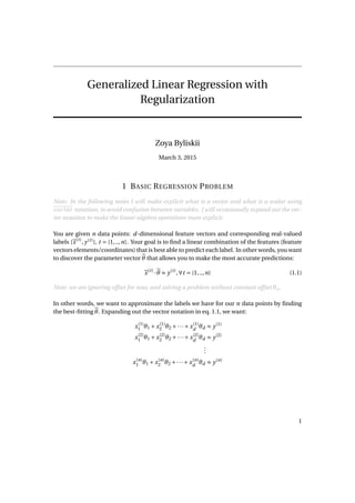
1. Generalized Linear Regression with
Regularization
Zoya Byliskii
March 3, 2015
1 BASIC REGRESSION PROBLEM
Note: In the following notes I will make explicit what is a vector and what is a scalar using
vector notation, to avoid confusion between variables. I will occasionally expand out the vec-
tor notation to make the linear algebra operations more explicit.
You are given n data points: d-dimensional feature vectors and corresponding real-valued
labels {x(t)
, y(t)
}, t = {1,..,n}. Your goal is to find a linear combination of the features (feature
vectors elements/coordinates) that is best able to predict each label. In other words, you want
to discover the parameter vector θ that allows you to make the most accurate predictions:
x(t)
·θ ≈ y(t)
,∀t = {1,..,n} (1.1)
Note: we are ignoring offset for now, and solving a problem without constant offset θo.
In other words, we want to approximate the labels we have for our n data points by finding
the best-fitting θ. Expanding out the vector notation in eq. 1.1, we want:
x(1)
1 θ1 + x(1)
2 θ2 +···+ x(1)
d
θd ≈ y(1)
x(2)
1 θ1 + x(2)
2 θ2 +···+ x(2)
d
θd ≈ y(2)
...
x(n)
1 θ1 + x(n)
2 θ2 +···+ x(n)
d
θd ≈ y(n)
1

2. This is just a linear system of n equations in d unknowns. So, we can write this in matrix form:






x(1)
x(2)
...
x(n)









θ1
...
θd


 ≈






y(1)
y(2)
...
y(n)






(1.2)
Or more simply as:
X θ ≈ y (1.3)
Where X is our data matrix.
Note: the horizontal lines in the matrix help make explicit which way the vectors are stacked
in the matrix. In this case, our feature vectors x(t)
make up the rows of our matrix, and the
individual features/coordinates are the columns.
Consider the dimensions of our system:
What happens if n = d?
X is square matrix, and as long as all the data points (rows) of X are linearly independent,
then X is invertible and we can solve for θ exactly:
θ = X −1
y (1.4)
Of course a θ that exactly fits all the training data is not likely to generalize to a test set (a
novel set of data: new feature vectors x(t)
). Thus we might want to impose some regulariza-
tion to avoid overfitting (will be discussed later in this document), or to subsample the data
or perform some cross-validation (leave out part of the training data when solving for the pa-
rameter θ).
2

3. What happens if n < d?
In this case, we have fewer data points than feature dimensions - less equations than un-
knowns. Think: how many degree-3 polynomials can pass through 2 points? An infinite
number. Similarly, in this case, we can have an infinite number of solutions. Our problem
is undefined in this case. What can we do? Well, we can collect more data, we can replicate
our existing data while adding some noise to it, or we can apply some methods of feature se-
lection (a research area in machine learning) to select out the features (columns of our data
matrix) that carry the most weight for our problem. We have to regularize even more severely
in this case, because there’s an infinite number of ways to overfit the training data.
What happens if n > d?
Now we have more data than features, so the more data we have, the less likely we are to
overfit the training set. In this case, we will not be able to find an exact solution: a θ that
satisfies eq. 1.1. Instead, we will look for a θ that is best in the least-squares sense. It turns
out, as we will see later in this document, that this θ can be obtained by solving the modified
system of equations:
X T
X θ = X T
y (1.5)
This is called the normal equations. Notice that X T
X is a square d ×d, invertible matrix 1
.
We can now solve for θ as follows:
θ = (X T
X )−1
X T
y (1.6)
Where (X T
X )−1
X T
is often denoted as X +
and is called the pseudoinverse of X .
1An easy-to-follow proof is provided here: <https://www.khanacademy.org/math/linear-algebra/
matrix_transformations/matrix_transpose/v/lin-alg-showing-that-a-transpose-x-a-is-invertible>
3

4. Let us now arrive at this solution by direct optimization of the least squares objective:
J(θ) =
1
n
n
t=1
1
2
y(t)
−θ · x(t)
2
(1.7)
Notice that this is just a way of summarizing the constraints in eq. 1.1. We want θ·x(t)
to come
as close as possible to y(t)
for all t, so we minimize the sum of squared errors.
Note: the 1
2 term is only for notational convenience (for taking derivatives). It is just a constant
scaling factor of the final θ we obtain. Also, the 1
n term is not important for this form of re-
gression without regularization, as it will cancel out. In the form with regularization, it just
rescales the regularization parameter by the amount of data points n (we’ll see this later in this
document). In any case, you might see formulations of regression with or without this term,
but this will not make a big difference to the general form of the problem.
We want to minimize J(θ), and so we set the gradient of this function to zero: ∇θ(J(θ)) = 0.
This is equivalent to solving the following system of linear equations:







∂
∂θ1
(J(θ))
∂
∂θ2
(J(θ))
...
∂
∂θd
(J(θ))







=






0
0
...
0






(1.8)
Let’s consider a single one of these equations: i.e. solve for a particular partial ∂
∂θi
(J(θ)). For
clarity, consider expanding the vector notation in 1.7:
J(θ) =
1
n
n
t=1
1
2
y(t)
− x(t)
1 θ1 + x(t)
2 θ2 +···+ x(t)
d
θd
2
(1.9)
Thus, by the chain rule:
∂
∂θi
(J(θ)) =
1
n
n
t=1
y(t)
− x(t)
1 θ1 + x(t)
2 θ2 +···+ x(t)
d
θd −x(t)
i
(1.10)
=
1
n
n
t=1
y(t)
− x(t)
T
θ −x(t)
i
(1.11)
Note: we just rewrote the dot product θ · x(t)
in equivalent matrix form: x(t)
T
θ because we
will be putting our whole system of equations in matrix form in the following calculations.
Since we want to set all the partials to 0, it follows that:
1
n
n
t=1
y(t)
− x(t)
T
θ −x(t)
i
= 0 (1.12)
1
n
n
t=1
x(t)
i
x(t)
T
θ =
1
n
n
t=1
x(t)
i
y(t)
(1.13)
4

5. So we can rewrite the system in eq. 1.14 as:









1
n
n
t=1 x(t)
1 x(t)
T
θ
1
n
n
t=1 x(t)
2 x(t)
T
θ
...
1
n
n
t=1 x(t)
d
x(t)
T
θ









=






1
n
n
t=1 x(t)
1 y(t)
1
n
n
t=1 x(t)
2 y(t)
...
1
n
n
t=1 x(t)
d
y(t)






(1.14)
Which is equivalent to the following condensed form:
1
n
n
t=1
x(t)
x(t)
T
θ =
1
n
n
t=1
x(t)
y(t)
(1.15)
Dropping the 1
n term:
n
t=1
x(t)
x(t)
T
θ =
n
t=1
x(t)
y(t)
(1.16)
In other words, this equation is what we obtain by setting ∇θ(J(θ)) = 0.
Let us write this equation out explicitly to see how we can rewrite it further in matrix form.
First, consider writing out the left-hand-size of eq. 1.16:






x(1)
1
x(1)
2
...
x(1)
d






x(1)
1 x(1)
2 ...x(1)
d
θ +






x(2)
1
x(2)
2
...
x(2)
d






x(2)
1 x(2)
2 ...x(2)
d
θ +...+






x(n)
1
x(n)
2
...
x(n)
d






x(n)
1 x(n)
2 ...x(n)
d
θ (1.17)
Convince yourself that this is just:


x(1)
x(2)
... x(n)









x(1)
x(2)
...
x(n)






θ (1.18)
These matrices should be familiar from before. We can rewrite eq. 1.18 as X T
X θ.
Next, consider writing out the right-hand-size of eq. 1.16:






x(1)
1
x(1)
2
...
x(1)
d






y(1)
+






x(2)
1
x(2)
2
...
x(2)
d






y(2)
+...+






x(n)
1
x(n)
2
...
x(n)
d






y(n)
(1.19)
5

6. Convince yourself that this is just:


x(1)
x(2)
... x(n)


 y (1.20)
Which is nothing more than X T
y.
Putting together eq. 1.18 and eq. 1.20, we get exactly eq. 1.5, and so:
θ = (X T
X )−1
X T
y
as the least-squares solution of our regression problem (no offset, no regularization).
2 REGRESSION WITH REGULARIZATION
If we overfit our training data, our predictions may not generalize very well to novel test data.
For instance, if our training data is somewhat noisy (real measurements are always somewhat
noisy!), we don’t want to fit our training data perfectly - otherwise we might generate very bad
predictions for real signal. It is worse to overshoot than undershoot predictions when errors
are measured by squared error. Being more guarded in how you predict, i.e., keeping θ small,
helps reduce generalization error. We can enforce the constraint to keep θ small by adding a
regularization term to 1.7:
J(θ) =
1
n
n
t=1
1
2
y(t)
−θ · x(t)
2
+
λ
2
θ 2
(2.1)
Since λ
2 θ 2
= λ
2 θ2
1 + λ
2 θ2
2 +···+ λ
2 θ2
d
this contributes a single additional term to eq. 1.11:
∂
∂θi
(J(θ)) =
1
n
n
t=1
y(t)
− x(t)
T
θ −x(t)
i
+λθi (2.2)
So similarly to eq. 1.13, setting the partial to zero:
1
n
n
t=1
x(t)
i
x(t)
T
θ+λθi =
1
n
n
t=1
x(t)
i
y(t)
(2.3)
Thus, collapsing the equations for all partials:
1
n
n
t=1
x(t)
x(t)
T
θ+λθ =
1
n
n
t=1
x(t)
y(t)
(2.4)
And in matrix form:
6

7. 1
n
X T
X θ+λθ =
1
n
X T
y (2.5)
1
n
X T
X +λI θ =
1
n
X T
y (2.6)
(2.7)
Which gives us the solution of our least-squares regression problem with regularization:
θ =
1
n
X T
X +λI
−1
1
n
X T
y
Note: You can see that the 1
n term was not dropped in the regularized form of the problem, but
is equivalent to a rescaling of λ.
Aside: how do we know 1
n X T
X +λI is invertible? Here is a rough proof outline:
• First note that X T
X is positive semidefinite
proof: uT
X T
Xu = ||Xu||2
≥ 0 so all eigenvalues must be ≥ 0
• The eigenvalues of X T
X +λI are µi +λ, where µi are eigenvalues of X T
X
proof: X T
Xu = µu implies (X T
X +λI)u = (µ+λ)u
• All eigenvalues of X T
X are strictly positive, so it must be invertible
proof: λ > 0, and so µi +λ > 0 for every i
3 REGRESSION WITH REGULARIZATION AND OFFSET
The offset parameter can be thought of as adjusting to the magnitude of the data. It is a
single scalar, and we do not want to penalize its size during regularization, because a large
offset might allow many of the other parameters to be much smaller and still provide a good
fit for the data. The calculation for the least-squares solution with regularization and offset is
similar to the calculation without offset.
J(θ) =
1
n
n
t=1
1
2
y(t)
− θ · x(t)
+θo
2
+
λ
2
θ 2
(3.1)
Setting ∇θ(J(θ)) = 0 as before, we have:
1
n
n
t=1
x(t)
x(t)
T
θ+
1
n
θo
n
t=1
x(t)
+λθ =
1
n
n
t=1
x(t)
y(t)
(3.2)
And in matrix form:
7

8. 1
n
X T
X θ+
1
n
θo X T
1+λθ =
1
n
X T
y (3.3)
1
n
X T
X +λ θ +
1
n
X T
1 θo =
1
n
X T
y (3.4)
Where 1 is the vector composed of all ones (here with dimension n×1), and so X T
1 = n
t=1 x(t)
.
We separately minimize J(θ) with respect to θo (which does not appear in the regularizer):
∂
∂θo
(J(θ)) =
1
n
n
t=1
y(t)
− x(t)
T
θ −θo (−1) (3.5)
Setting this partial to 0 we get:
θo =
1
n
n
t=1
y(t)
− x(t)
T
θ (3.6)
=
1
n
yT
1−
1
n
X θ
T
1 (3.7)
Note that we now have 2 equations (3.4 and 3.7) in 2 unknowns: θ and θo that can be solved
algebraically.
4 ADDITIONAL RESOURCES
• Matrix cookbook: <http://www.mit.edu/~wingated/stuff_i_use/matrix_cookbook.
pdf>.
• Matrix approach to linear regression with a statistical perspective: <http://www.maths.
qmul.ac.uk/~bb/SM_I_2013_LecturesWeek_6.pdf>.
8