Downloaded 902 times
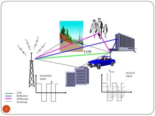
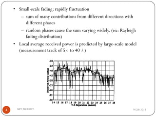
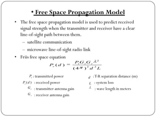
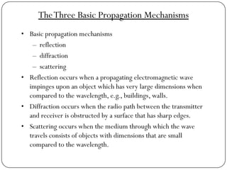
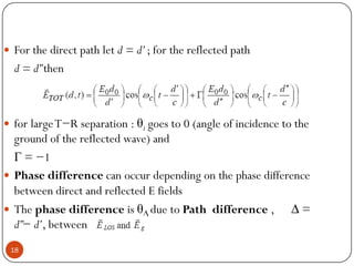
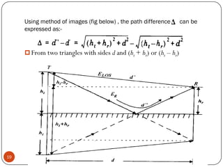
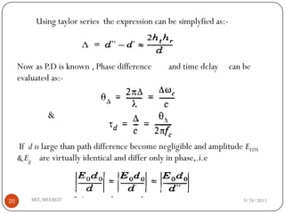
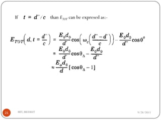
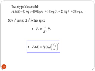
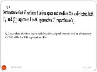
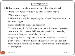
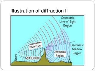
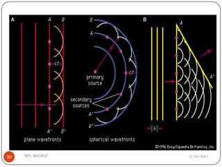
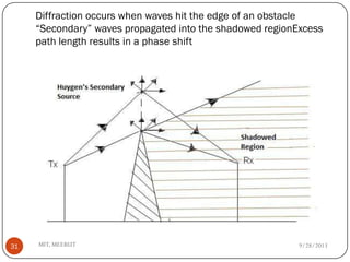
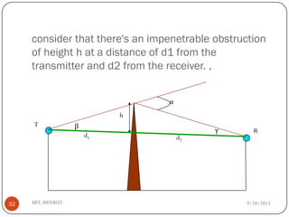
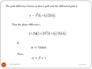
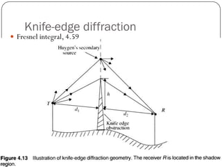
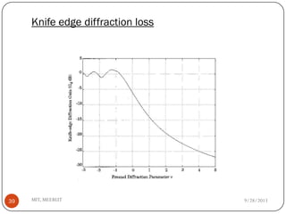
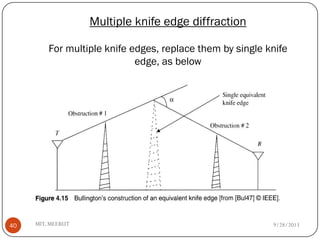
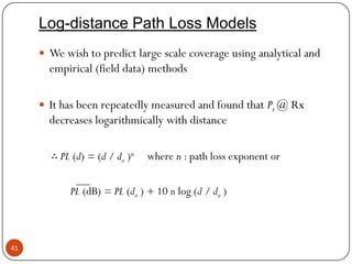
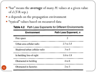
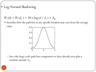

The document discusses various propagation mechanisms that affect radio signals, including reflection, diffraction, scattering, and their effects on signal strength over distance. It also covers propagation models like free space path loss, two-ray ground reflection model, and log-distance path loss for estimating average received signal power at a given distance. Fresnel zones and knife-edge diffraction are explained as factors in signal propagation around obstructions. Log-normal shadowing is described as a statistical model to account for variations from the average path loss.