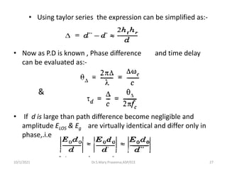
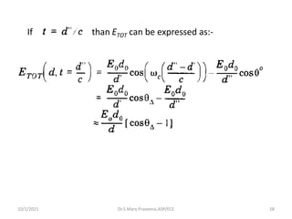
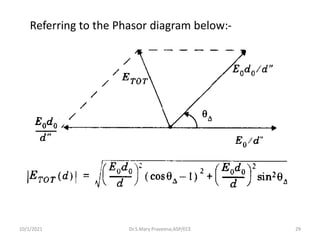
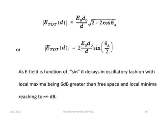
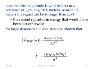
The document discusses various aspects of wireless channels including:
1) Large-scale path loss models like the free space and two-ray models for estimating mean signal strength over distance.
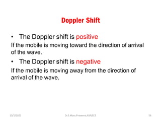
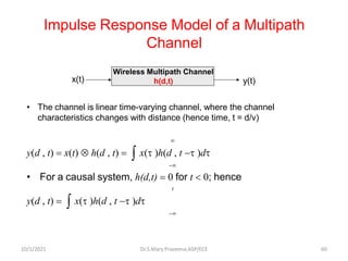
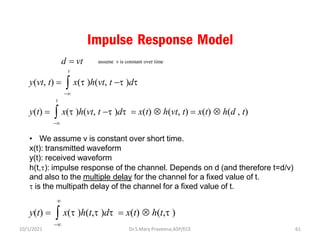
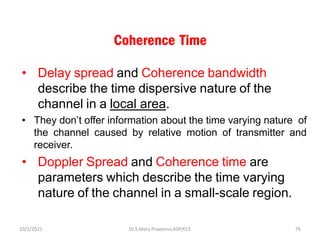
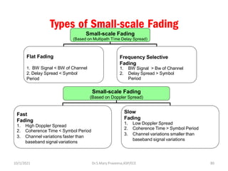
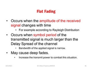
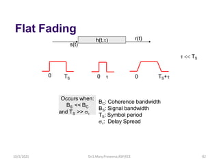
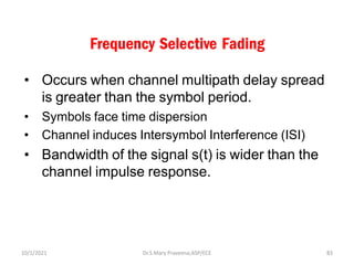
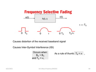
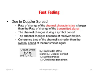
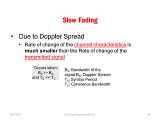
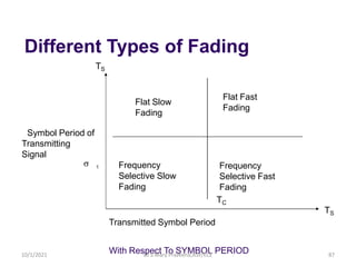
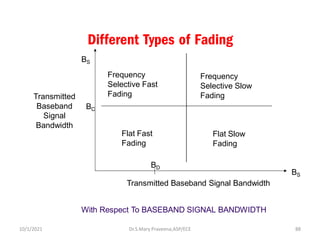
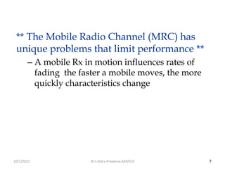
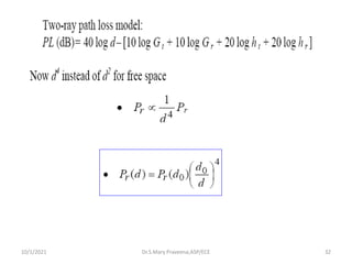
2) Small-scale fading parameters caused by multipath time delay and Doppler spread which can result in flat or frequency selective fading.
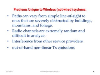
3) Characteristics of the mobile radio channel that introduce problems like fading and interference not seen in wired channels.

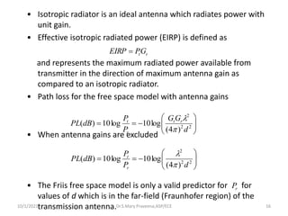
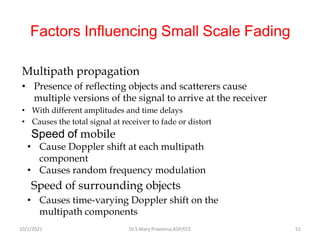
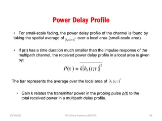
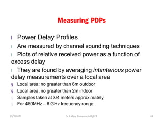
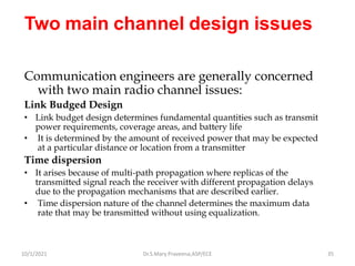
![• Expressing the received power in dBm and dBW
l Pr(d) (dBm) = 10 log [Pr(d0)/0.001W] + 20log(d0/d)
where d >= d0 >= df and Pr(d0) is in units of watts.
l Pr(d) (dBW) = 10 log [Pr(d0)/1W] + 20log(d0/d)
where d >= d0 >= df and Pr(d0) is in units of watts.
• Reference distance d0 for practical systems:
l For frequencies in the range 1-2 GHz
• 1 m in indoor environments
• 100m-1km in outdoor environments
Dr.S.Mary Praveena,ASP/ECE 18
10/1/2021](https://image.slidesharecdn.com/wirelesschannels-converted-1-211001094238/85/Wireless-channels-18-320.jpg)
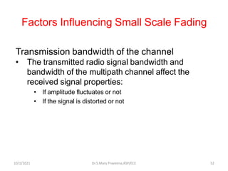
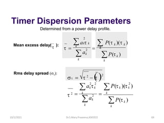
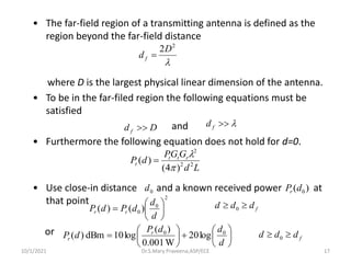
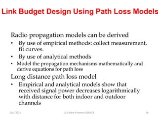
![Solution
A)
Pt(W) is 50W.
Pt(dBm) = 10log[Pt(mW)/1mW)]
Pt(dBm) = 10log(50x1000)
Pt(dBm) = 47 dBm
B)
Pt(dBW) = 10log[Pt(W)/1W)]
Pt(dBW) = 10log(50)
Pt(dBW) = 17 dBW
Dr.S.Mary Praveena,ASP/ECE 20
10/1/2021](https://image.slidesharecdn.com/wirelesschannels-converted-1-211001094238/85/Wireless-channels-20-320.jpg)
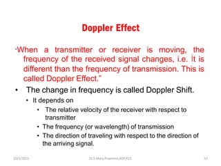
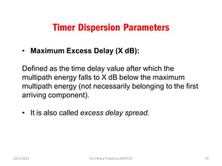
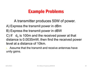
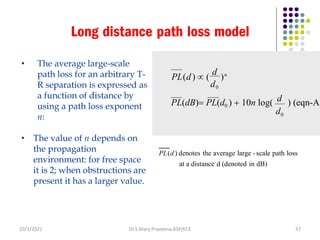
![Solution
c) Pr(d) = Pr(d0)(d0/d)2
Substitute the values into the equation:
lPr(10km) = Pr(100m)(100m/10km)2
Pr(10km) = 0.0035mW(10-4)
Pr(10km) = 3.5x10⁻¹⁰W
Pr(10km) [dBm] = 10log(3.5x10⁻¹⁰W/1mW)
= 10log(3.5x10⁻⁷)
= -64.5dBm
Dr.S.Mary Praveena,ASP/ECE 21
10/1/2021](https://image.slidesharecdn.com/wirelesschannels-converted-1-211001094238/85/Wireless-channels-21-320.jpg)
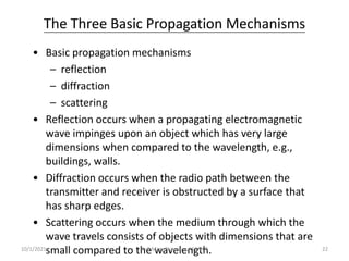
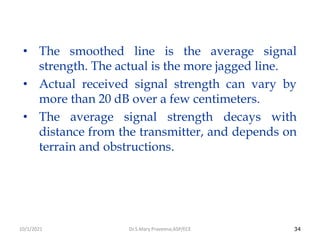
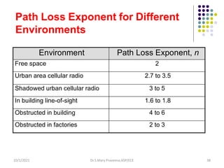
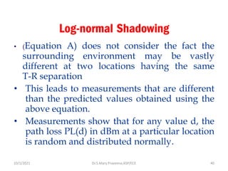
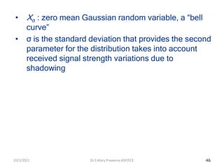
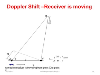
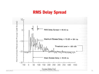
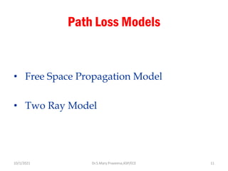
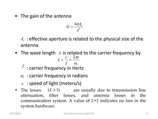
![PL(d ) denotes the average large-scale path loss (in dB) at a distance d.
X is a zero-mean Gaussian (normal) distributed random variable (in dB)
with standard deviation (also in dB).
PL(d0 ) is usually computed assuming free space propagation model between
transmitter and d0 (or by measurement).
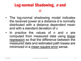
Equation B takes into account the shadowing affects due to
cluttering on the propagation path. It is used as the propagation model for
log-normal shadowing environments.
Log-normal Shadowing- Path Loss
PL(d)[dB] = PL(d0 ) +10nlog(
d
) + X
Then adding this random factor:
PL(d)[dB] = PL(d) + X
d
0
Equation B
Dr.S.Mary Praveena,ASP/ECE 41
10/1/2021](https://image.slidesharecdn.com/wirelesschannels-converted-1-211001094238/85/Wireless-channels-41-320.jpg)
![Log-normal Shadowing- Received Power
• The received power in log-normal shadowing
environment is given by the following formula
(derivable from Equation B)
l The antenna gains are included in PL(d).
Pr (d)[dBm] = Pt [dBm]− PL(d0 )[dB]+10nlog(
d
) + X [dB]
Pr (d)[dBm] = Pt [dBm]− PL(d)[dB]
0
d
Dr.S.Mary Praveena,ASP/ECE 42
10/1/2021](https://image.slidesharecdn.com/wirelesschannels-converted-1-211001094238/85/Wireless-channels-42-320.jpg)