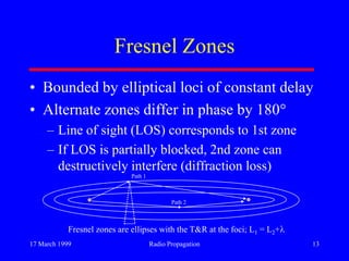
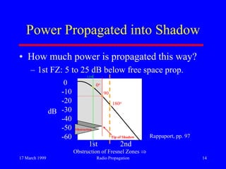
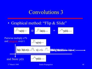
Downloaded 196 times
(
What is dB?](https://image.slidesharecdn.com/radiopropagation-140328202308-phpapp01/85/Radio-propagation-20-320.jpg)

![17 March 1999 Radio Propagation 49
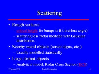
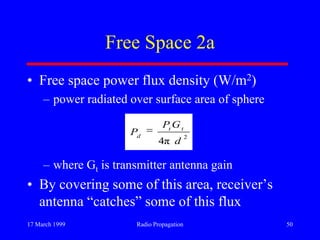
Scattering 2
• hc is the critical height of a protrusion to
result in scattering.
• RCS: ratio of power density scattered to receiver
to power density incident on the scattering object
– Wave radiated through free space to scatterer and reradiated:
)sin( θ8
λ
i
c
h
)log(20)log(20)π4log(30
]dB[)λlog(20)dBi()dBm()dBm(
2
RT
TTR
dd
mRCSGPP](https://image.slidesharecdn.com/radiopropagation-140328202308-phpapp01/85/Radio-propagation-49-320.jpg)

![17 March 1999 Radio Propagation 53
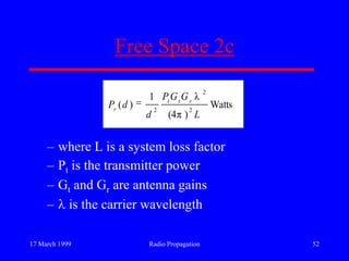
LNSM 2
• PL(d)[dB] = PL(d0) +10nlog(d/d0)+ X
– where X is a zero-mean Gaussian RV (dB)
• and n computed from measured data,
based on linear regression](https://image.slidesharecdn.com/radiopropagation-140328202308-phpapp01/85/Radio-propagation-53-320.jpg)
![17 March 1999 Radio Propagation 60
dB 2
• Ex: Attenuation from transmitter to receiver.
– PT=100, PR=10
– attenuation is ratio of PT to PR
– [PT/PR]dB = 10 log(PT/PR) = 10 log(10) = 10 dB
• Useful numbers:
– [1/2]dB -3 dB
– [1/1000]dB = -30 dB](https://image.slidesharecdn.com/radiopropagation-140328202308-phpapp01/85/Radio-propagation-60-320.jpg)
![17 March 1999 Radio Propagation 61
dB 3
• dB can express ratios, but what about
absolute quantities?
• Similar units reference an absolute quantity
against a defined reference.
– [n mW]dBm = [n/mW]dB
– [n W]dBW = [n/W]dB
• Ex: [1 mW]dBW = -30 dBW](https://image.slidesharecdn.com/radiopropagation-140328202308-phpapp01/85/Radio-propagation-61-320.jpg)
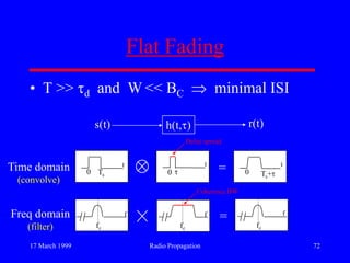
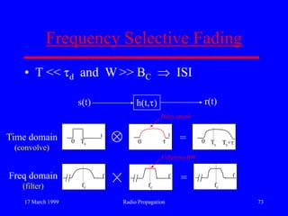
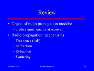
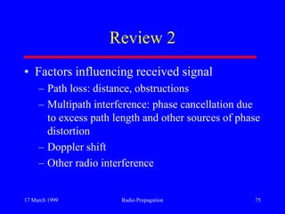

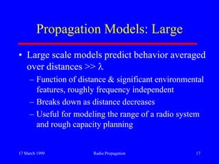
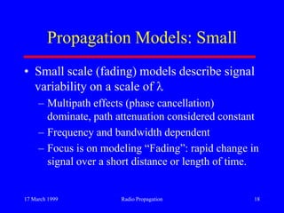
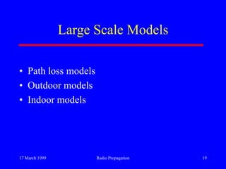
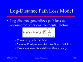
This document discusses radio propagation and propagation models. It begins with an introduction to radio and propagation mechanisms like free space propagation, refraction, diffraction, and scattering. It then discusses the objective of developing propagation models to predict signal strength at a receiver. The document outlines that propagation models are specialized based on scale, environment, and application. It covers large-scale path loss models and small-scale fading models. It discusses specific propagation mechanisms and models like free space, log-distance path loss, ground reflection, hilly terrain, indoor models, and statistical fading models.