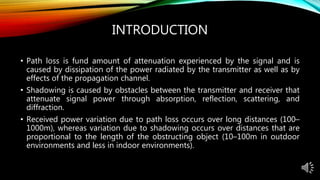
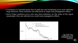
The document discusses path loss and shadowing in wireless communication, detailing their causes and effects on signal strength as it propagates through various environments. It covers various models for calculating path loss, including empirical models like the Okumura and Hata models, as well as simplified approaches for practical system design. Additionally, the document addresses shadow fading and how it can be combined with path loss models to more accurately predict received power variations.

1. PATH LOSS AND SHADOWING
Presented by
Yash Gupta
A presentation on

2. CONTENT
1. Introduction
2. Transmit and Receive Model
3. Free-Space Path Loss
4. Ray Tracing
5. Empirical Path-Loss Models
6. Simplified Path-Loss Model
7. Shadow Fading
8. Combined Path Loss and Shadowing

3. INTRODUCTION
• Path loss is fund amount of attenuation experienced by the signal and is
caused by dissipation of the power radiated by the transmitter as well as by
effects of the propagation channel.
• Shadowing is caused by obstacles between the transmitter and receiver that
attenuate signal power through absorption, reflection, scattering, and
diffraction.
• Received power variation due to path loss occurs over long distances (100–
1000m), whereas variation due to shadowing occurs over distances that are
proportional to the length of the obstructing object (10–100m in outdoor
environments and less in indoor environments).

4. • If variations in received power due to path loss and shadowing occur over relatively
large distances, these variations are referred to as large-scale propagation effects.
• And if these variations occur over very short distances, on the order of the signal
wavelength, then are referred to as small-scale propagation effects.
Fig. Path loss,
shadowing, and
multipath versus
distance.

5. TRANSMIT AND RECEIVE MODEL
• When the transmitter or receiver is moving, the received signal will have a Doppler
shift of fD = v cos θ/λ associated with it, where θ is the arrival angle of the received
signal relative to the direction of motion, v is the receiver velocity toward the
transmitter in the direction of motion, and λ = c/fc is the signal wavelength.
• The geometry associated with the
Doppler shift is shown in Figure

6. • The linear path loss of the channel is defined as the ratio of transmit power
to receive power:
PL =
𝑃𝑡
𝑃𝑟
• Where, signal of power Pt is transmitted through a given channel with
corresponding received signal r(t) of power Pr , and Pr is averaged over any
random variations due to shadowing.
• The path loss of the channel as the value of the linear path loss in decibels is
PL dB = 10log10
𝑃𝑡
𝑃𝑟
dB

7. FREE-SPACE PATH LOSS
• When there are no obstructions between the transmitter and receiver and that the signal
propagates along a straight line between the two. The channel model associated with this
transmission is called a line-of-sight (LOS) channel, and the corresponding received signal is
called the LOS signal or ray.
• Free-space path loss is defined as the path loss of the free-space model:
PL dB = 10log10
𝑃𝑡
𝑃𝑟
= - 10log10
𝐺 𝑙 𝜆2
4𝜋𝑑 2
• The free-space path gain is thus
PG = -PL = 10log10
𝐺 𝑙 𝜆2
4𝜋𝑑 2
where G𝑙 is the product of the transmit and receive antenna field radiation patterns in the LOS
direction.

8. RAY TRACING
• In ray tracing, there is a finite number
of reflectors with known location and
dielectric properties.
• Ray-tracing techniques approximate
the propagation of electromagnetic
waves.
• Thus, the effects of reflection,
diffraction, and scattering on the wave
front are approximated using simple
geometric equations instead of
Maxwell’s more complex wave
equations.
• E.g. Two-Ray Model, Ten-Ray Model

9. TWO-RAY MODEL
• The two-ray model is used when a single ground reflection dominates the multipath
effect as shown in the figure.
• The received signal consists of two components: the LOS component or ray, which is
just the transmitted signal propagating through free space, and a reflected
component or ray, which is the transmitted signal reflected off the ground.

10. • For asymptotically large d, x + x’ ≈ 𝑙 ≈ d,
the received signal power is
approximately
Pr =
𝐺 𝑙ℎ 𝑡ℎ 𝑟
𝑑2
2
Pt
Where d denotes the horizontal
separation of the antennas, ht the
transmitter height, and hr the receiver
height.
• Figure shows Received power versus
distance for two-ray model.

11. EMPIRICAL PATH-LOSS MODELS
• In these models, measurements of Pr/Pt as a function of distance include the effects
of path loss, shadowing, and multipath.
• In order to remove multipath effects, empirical measurements for path loss typically
average their received power measurements and the corresponding path loss at a
given distance over several wavelengths.
• This average path loss is called the local mean attenuation (LMA) at distance d.
• Thus, the empirical path loss PL(d ) for a given environment is defined as the average
of the LMA measurements at distance d averaged over all available measurements
in the given environment.

12. OKUMURA MODEL
• One of the most common models for signal prediction in large urban macro cells is
the Okumura model.
• This model is applicable over distances of 1–100 km and frequency ranges of 150–
1500 MHz.
• Okumura used extensive measurements of base station-to-mobile signal
attenuation throughout Tokyo to develop a set of curves giving median attenuation
relative to free space of signal propagation in irregular terrain.
• The empirical path-loss formula of Okumura at distance d parameterized by the
carrier frequency fc is given by
PL(d) dB = L(fc, d) + Aμ(fc, d) − G(ht) − G(hr) − GAREA

13. HATA MODEL
• The Hata model is an empirical formulation of the graphical path-loss data provided
by Okumura and is valid over roughly the same range of frequencies, 150–1500
MHz.
• This empirical model simplifies calculation of path loss.
• The standard formula for empirical path loss in urban areas under the Hata model is
PL,urban(d) dB = 69.55 + 26.16 log10( fc ) −13.82 log10( ht ) − a( hr ) + (44.9 − 6.55 log10( ht
)) log10( d )
Where a(hr) is a correction factor for the mobile antenna height based on the size of
the coverage area.
a( hr ) = (1.1log10( fc ) − 0.7)hr − (1.56 log10( fc ) − 0.8) dB

14. • Unlike the Okumura model, the Hata model does not provide for any path-
specific correction factors.
• The Hata model well approximates the Okumura model for distances d > 1
km.
• Hence it is a good model for first-generation cellular systems, but it does not
model propagation well in current cellular systems with smaller cell sizes and
higher frequencies. Indoor environments are also not captured by the Hata
model.

15. SIMPLIFIED PATH-LOSS MODEL
• Simplified path- loss model captures the essence of signal propagation without
resorting to complicated path-loss models, which are only approximations to the
real channel anyway.
• Thus, the following simplified model for path loss as a function of distance is
commonly used for system design:
Pr = PtK
𝑑0
𝑑
𝛾
• The dB attenuation is thus
Pr dBm = Pt dBm + K dB - 10𝛾log10
𝑑0
𝑑
• Where K is a unitless constant, d0 is a reference distance for the antenna far field,
and γ is the path-loss exponent.

16. SHADOW FADING
• The most common model for the additional attenuation where the location, size,
and dielectric properties of the blocking objects – as well as the changes in
reflecting surfaces and scattering objects causes the random attenuation is log-
normal shadowing.
• This model has been empirically confirmed to model accurately the variation in
received power in both outdoor and indoor radio propagation environments.
• Log-normal distribution is:
where ξ = 10/ln10, μψdB is the mean of ψdB = 10 log10 ψ in dB, and σψdB is the standard
deviation of ψdB.

17. COMBINED PATH LOSS AND SHADOWING
• Models for path loss and shadowing can be superimposed to capture power falloff
versus distance along with the random attenuation about this path loss from
shadowing.
• In this combined model, average dB path loss (μψdB) is characterized by the path-
loss model while shadow fading, with a mean of 0 dB.
• For this combined model, the ratio of received to transmitted power in dB is given
by:
𝑃𝑟
𝑃𝑡
dB = 10 log10 K −10γ log10
𝑑
𝑑0
- ψdB
where ψdB is a Gauss-distributed random variable with mean zero and variance σ2
ψdB

18. REFERENCES
[1] Andrea Goldsmith, “Wireless Communications”, 2005
[2] Sanjay Kumar, “Wireless Communication the fundamental concept and advanced
concepts”
[3] T Sun-Kuk Noh, and Dong You Choi, "Propagation Model in Indoor and Outdoor
for the LTE Communications”, International Journal of Antennas and Propagation,
2019
[4] T. S. Rappaport, et.al., "Overview of millimeter wave communications for fifth-
generation (5G) wireless networks-with a focus on propagation models," IEEE
Transactions on Antennas and Propagation, 2017

19. THANK YOU