This document provides an introduction and overview of the book "HSDPA/HSUPA for UMTS: High Speed Radio Access for Mobile Communications". The book is edited by Harri Holma and Antti Toskala of Nokia Networks, Finland. It covers the standardization of HSDPA and HSUPA in 3GPP, the key technologies and principles of HSDPA and HSUPA including new physical channels and protocols, radio resource management, performance metrics such as bit rates and capacity, and applications over HSPA such as voice-over-IP.
![2 HSDPA/HSUPA for UMTS
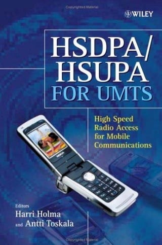
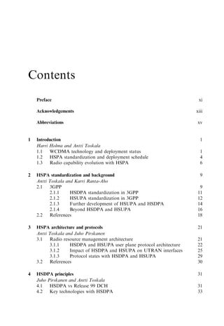
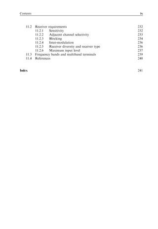
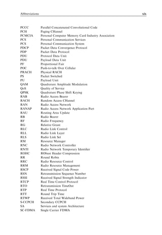
WCDMA subscribers globally February 2006
60
50
40
Million
30
20
10
0
b 04
y 4
b 05
y 5
ay 4
ay 5
S e Jul 0 4
S e Jul 0 5
ch 4
ov ber 4
ch 5
ov er 5
06
n u 00
n u 00
0
0
0
b 0
0
0
em 20
em 20
20
20
em 0
em 0
20
20
M 20
M 20
20
Ja er 2
Ja er 2
pt y 2
pt y 2
ry
ar
ar
ua
ar
ar
M
M
n
Ja
N
N
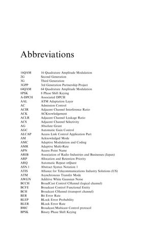
Figure 1.1 3G WCDMA subscriber growth monthly.
USA
2003 2004 2005
Figure 1.2 Evolution of Nokia 3G terminal offering.
[www.nokia.com]
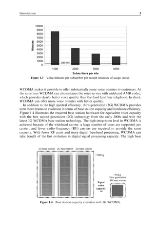
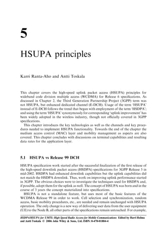
the operator in that it enables data but also improves basic voice. The offered voice
capacity is very high because of interference control mechanisms including frequency
reuse of 1, fast power control and soft handover. Figure 1.3 shows the estimated number
of voice minutes per subscriber per month that can be supported with a two-carrier,
three-sector, 2 þ 2 þ 2 WCDMA site depending on the number of subscribers in the site
coverage area. Adaptive multi-rate (AMR) 5.9-kbps voice codec is assumed in the
calculation. With 2000 subscribers in each base station coverage area, 4300 minutes
per month can be offered to each subscriber, while with 4000 subscribers even more than
2100 minutes can be used. These capacities include both incoming and outgoing minutes.
Global average usage today is below 300 minutes per month. This calculation shows that](https://image.slidesharecdn.com/wileyhsdpahsupaforumts-12712250730845-phpapp02/85/Hsdpa-Hsupa-For-Umts-21-320.jpg)
![Introduction 5
f2
f2
f1
f1
Base RNC 3G-SGSN GGSN
station
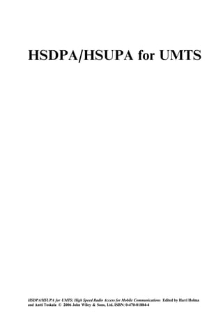
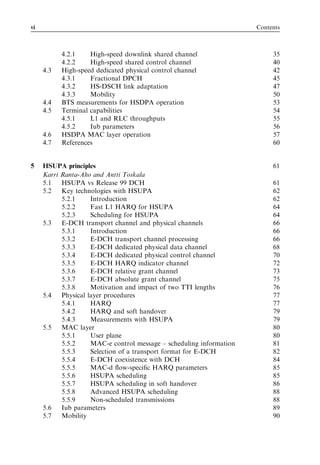
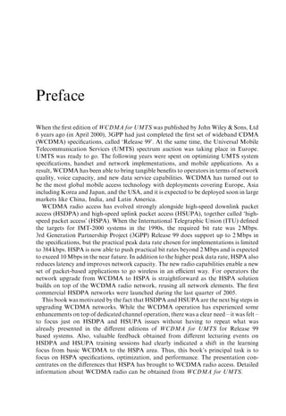
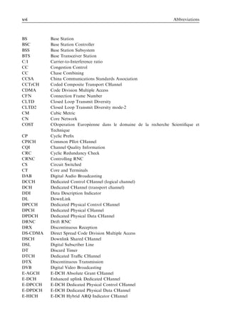
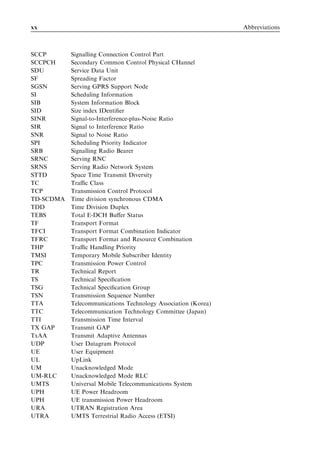
Figure 1.7 HSPA deployment with (f2) new carrier deployed with HSPA and (f1) carrier shared
between WCDMA and HSPA.
in the radio network including base stations, Radio Network Controller (RNC),
Serving GPRS Support Node (SGSN) and Gateway GPRS Support Node (GGSN).
WCDMA and HSPA are also sharing the base station sites, antennas and antenna lines.
The upgrade from WCDMA to HSPA requires new software package and, potentially,
some new pieces of hardware in the base station and in RNC to support the higher data
rates and capacity. Because of the shared infrastructure between WCDMA and HSPA,
the cost of upgrading from WCDMA to HSPA is very low compared with building a
new standalone data network.
The first HSDPA terminals are data cards providing fast connectivity for laptops. An
example terminal – Sierra Wireless AirCard 850 – is shown in Figure 1.8 providing 1.8-
Mbps downlink and 384-kbps uplink peak data rates.
HSDPA terminal selection will expand beyond PCMCIA cards when integrated
HSDPA mobile terminals are available during 2006. It is expected that HSPA will be
a standard feature of most 3G terminals after some years in the same way as Enhanced
Data Rates for GSM Evolution (EDGE) capability is included in most GSM/GPRS
terminals. HSDPA will also be integrated to laptop computers in the future, as is
indicated already by some of the laptop manufacturers.
Figure 1.8 Example of first-phase HSDPA terminal.
[Courtesy of Sierra Wireless]](https://image.slidesharecdn.com/wileyhsdpahsupaforumts-12712250730845-phpapp02/85/Hsdpa-Hsupa-For-Umts-24-320.jpg)
![6 HSDPA/HSUPA for UMTS
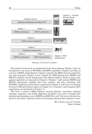
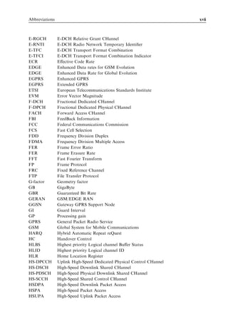
1.3 Radio capability evolution with HSPA
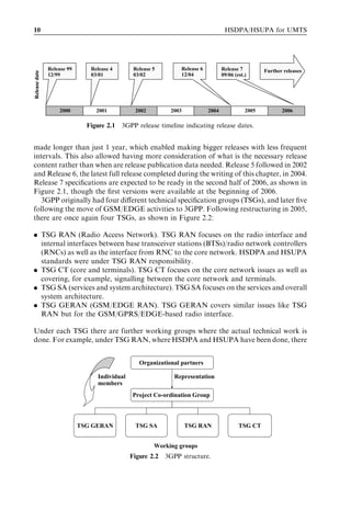
The performance of the radio system defines how smoothly applications can be used over
the radio network. The key parameters defining application performance include data
rate and network latency. There are applications that are happy with low bit rates of a
few tens of kbps but require very low delay, like voice-over-IP (VoIP) and real time action
games. On the other hand, the download time of a large file is only defined by the
maximum data rate, and latency does not play any role. GPRS Release 99 typically
provides 30–40 kbps with latency of 600 ms. EGPRS Release 4 pushes the bit rates 3–4
times higher and also reduces latency below 300 ms. The EGPRS data rate and latency
allow smooth application performance for several mobile-based applications including
Wireless Application Protocol (WAP) browsing and push-to-talk.
WCDMA enables peak data rates of 384 kbps with latency 100–200 ms, which makes
Internet access close to low-end digital subscriber line (DSL) connections and provides
good performance for most low-delay Internet Protocol (IP) applications as well.
HSPA pushes the data rates up to 1–2 Mbps in practice and even beyond 3 Mbps in
good conditions. Since HSPA also reduces network latency to below 100 ms, the end user
experienced performance is similar to the fixed line DSL connections. No or only little
effort is required to adapt Internet applications to the mobile environment. Essentially,
HSPA is a broadband access with seamless mobility and extensive coverage. Radio
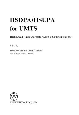
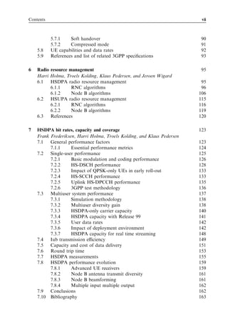
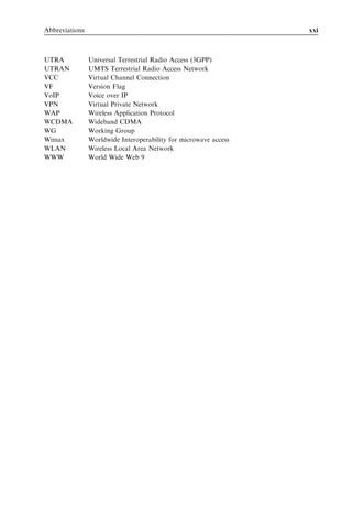
capability evolution from GPRS to HSPA is illustrated in Figure 1.9.
HSPA was initially designed to support high bit rate non-real time services. The
simulation results show, however, that HSPA can provide attractive capacity also for
low bit rate low-latency applications like VoIP. 3GPP Releases 6 and 7 further improve
the efficiency of HSPA for VoIP and other similar applications.
Typical end user bit
rates in macro cells
[kbps]
3
Mbps HSPA
1
Mbps
WCDMA
300
kbps
EGPRS
100
kbps
GPRS
30
kbps
600 300 0
Round trip time [ms]
Figure 1.9 Radio capability evolution.](https://image.slidesharecdn.com/wileyhsdpahsupaforumts-12712250730845-phpapp02/85/Hsdpa-Hsupa-For-Umts-25-320.jpg)
![Introduction 7
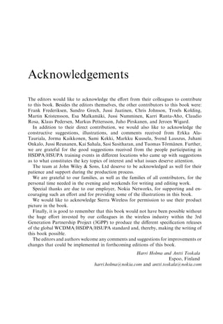
Cell capacity [per sector per 5 MHz]
5000
4500 Downlink
Uplink
4000
3500
3000
kbps
2500
2000
1500
1000
500
0
WCDMA HSPA Basic HSPA Enhanced
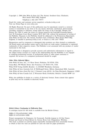
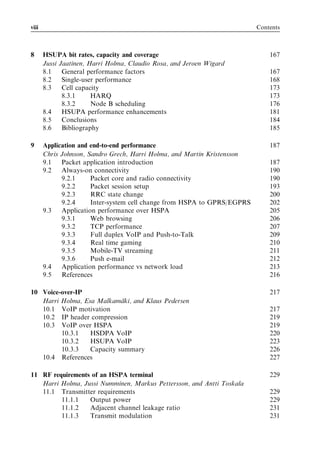
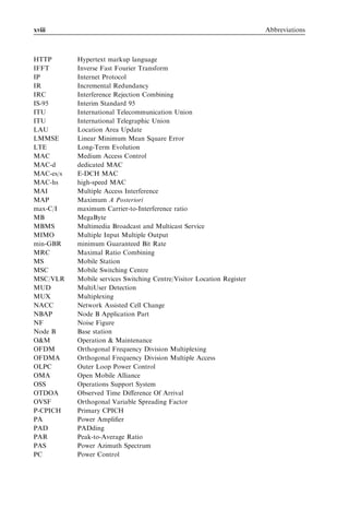
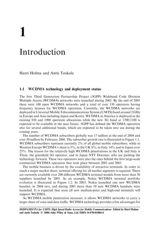
Figure 1.10 Capacity evolution with HSPA.
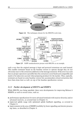
Higher cell capacity and higher spectral efficiency are required to provide higher data
rates and new services with the current base station sites. Figure 1.10 illustrates the
estimated cell capacity per sector per 5 MHz with WCDMA, with basic HSPA and with
enhanced HSPA in the macro-cell environment. Basic HSPA includes a one-antenna
Rake receiver in the terminals and two-branch antenna diversity in the base stations.
Enhanced HSPA includes two-antenna equalizer mobiles and interference cancellation
in the base station. The simulation results show that HSPA can provide substantial
capacity benefit. Basic HSDPA offers up to three times WCDMA downlink capacity,
and enhanced HSDPA up to six times WCDMA. The spectral efficiency of enhanced
HSDPA is close to 1 bit/s/Hz/cell. The uplink capacity improvement with HSUPA is
estimated between 30% and 70%. HSPA capacity is naturally suited for supporting not
only symmetric services but also asymmetric services with higher data rates and volumes
in downlink.](https://image.slidesharecdn.com/wileyhsdpahsupaforumts-12712250730845-phpapp02/85/Hsdpa-Hsupa-For-Umts-26-320.jpg)
![2
HSPA standardization
and background
Antti Toskala and Karri Ranta-Aho
This chapter introduces the standardization framework around high-speed downlink
packet access (HSDPA) and high-speed uplink packet access (HSUPA) and presents
the standardization schedule and future development for HSDPA and HSUPA currently
on-going. Also the developments beyond HSDPA and HSUPA are introduced at the end
of this chapter.
2.1 3GPP
The 3rd Generation Partnership Project (3GPP) is the forum [1] where standardization is
handled for HSDPA and HSUPA, as well as has been handled from the first wideband
code division multiple access (WCDMA) specification release. Further, 3GPP also has
responsibility for Global System for Mobile Communications (GSM)/Enhanced Data
Rates for Global Evolution (EDGE) standardization. The background of 3GPP is in the
days when WCDMA technology was being standardized following technology selections
in different regions during 1997. Following that, WCDMA was chosen in several places
as the basis for third-generation mobile communication systems and there was regional
activity in several places around the same technological principles. It became evident,
however, that this would not lead to a single global standard aligned down to bit level
details. Thus, at the end of 1998 the US, Europe, Korea and Japan joined forces and
created 3GPP. China followed a bit later. Note also that the related standardization
organization, although marked as regional, usually had members from other countries/
regions as well.
The first major milestone was reached at the end of 1999 when Release 99 specifications
were published, containing the first full series of WCDMA specifications. Release 4
specifications followed in early 2001. The working method had been moved between
Release 99 and Release 4 away from the yearly ‘release’ principle. The release cycle was
HSDPA/HSUPA for UMTS: High Speed Radio Access for Mobile Communications Edited by Harri Holma
and Antti Toskala © 2006 John Wiley & Sons, Ltd. ISBN: 0-470-01884-4](https://image.slidesharecdn.com/wileyhsdpahsupaforumts-12712250730845-phpapp02/85/Hsdpa-Hsupa-For-Umts-27-320.jpg)
![HSPA standardization and background 11
are five working groups (WGs) as follows:
. TSG RAN WG1: responsible for physical layer aspects;
. TSG RAN WG2: responsible for layer 2 and 3 aspects;
. TSG RAN WG3: responsible for RAN internal interfaces;
. TSG RAN WG4: responsible for performance and radio frequency (RF) require-
ments;
. TSG RAN WG5: responsible for terminal testing.
The 3GPP membership is organized through organizational partners. Individual
companies need to be members of one of the organizational partners, and based on
this membership there is the right to participate in 3GPP activity. The following are the
current organizational partners:
. Alliance for Telecommunications Industry Solutions (ATIS) from the US.
. European Telecommunications Standards Institute (ETSI) from Europe.
. China Communications Standards Association (CCSA) from China.
. Association of Radio Industries and Businesses (ARIB) from Japan.
. Telecommunication Technology Committee (TTC) from Japan.
. Telecommunications Technology Association (TTA) from South Korea.
3GPP creates the technical content of the specifications, but it is the organizational
partners that actually publish the work. This enables having identical sets of specifi-
cations in all regions, thus ensuring roaming across continents. In addition to the
organizational partners, there are also so-called market representation partners, such
as the UMTS Forum, part of 3GPP.
The work in 3GPP is based around work items, though small changes can be intro-
duced directly as ‘change requests’ against specification. With bigger items a feasibility
study is done usually before rushing in to making actual changes to the specifications.
2.1.1 HSDPA standardization in 3GPP
When Release 99 was completed, HSDPA or HSUPA were not yet on the agenda.
During 2000, while also making corrections to WCDMA Release 99 and working on
Release 4 to include, for example, TD-SCDMA, it became obvious that some improve-
ments for packet access would be needed. To enable such an evolution, a feasibility study
(study item) for HSDPA was started in March 2000. As shown in the study item proposal
[2], the work was initiated in line with 3GPP principles, having at least four supporting
companies. The companies supporting the start of work on HSDPA were Motorola and
Nokia from the vendor side and BT/Cellnet, T-Mobile and NTT DoCoMo from the
operator side, as indicated in [2].
The feasibility study was finalized for the TSG RAN plenary for March 2001 and the
conclusions reported in [3] were such that there was clear benefit to be seen with the
solutions studied. In the HSDPA study item there were issues studied to improve
the downlink packet data transmission over Release 99 specifications. Topics such as
physical layer retransmissions and BTS-based scheduling were studied as well as adaptive](https://image.slidesharecdn.com/wileyhsdpahsupaforumts-12712250730845-phpapp02/85/Hsdpa-Hsupa-For-Umts-29-320.jpg)
![12 HSDPA/HSUPA for UMTS
coding and modulation. The study also included some investigations for multi-antenna
transmission and reception technology, titled ‘multiple input multiple output’ (MIMO),
as well as on fast cell selection (FCS).
As the feasibility study clearly demonstrated that significant improvement was possible
to achieve and with reasonable complexity, it was clear to proceed for an actual work
item to develop specifications. When the work item was set up [4] the scope of the work
was in line with the study item, but MIMO was taken as a separate work item and a
separate feasibility study on FCS was started. For the HSDPA work item there was
wider vendor support and the actual work item was supported from the vendor side by
Motorola, Nokia and Ericsson. During the course of work, obviously much larger
numbers of companies contributed technically to the progress.
When Release 5 specifications with HSDPA were released 1 year later – in March
2002 – there were clearly still corrections to do in HSDPA, but the core functionality
was already in the physical layer specifications. The work was partly slowed down by the
parallel corrections activity needed for the Release 99 terminals and networks being
rolled out. Especially with protocol aspects, intensive testing tends to reveal details that
need corrections and clarifications in the specifications and this was the case with
Release 99 devices preceding the start of commercial operations in Europe in the
second half of 2002. The longest time was taken for HSDPA protocol parts, on
which backward compatibility was started in March 2004.
From the other topics that relate to HSDPA, the MIMO work item did not complete in
the Release 5 or Release 6 time frame, and it is still under discussion whether there is
sufficient merit for the introduction of it – as covered in the Release 7 topic listing. The
feasibility study on FCS concluded that the benefits were limited to the extent that
additional complexity would not be justified, thus no work item was created around FCS
after the study was closed. While focus was on the frequency division duplex (FDD) side,
time division duplex (TDD) was also covered in the HSDPA work item to include similar
solutions in both TDD modes (narrowband and wideband TDD).
2.1.2 HSUPA standardization in 3GPP
Although HSUPA is a term used broadly in the market, in 3GPP the standardization for
HSUPA was done under the name ‘enhanced uplink dedicated channel’ (E-DCH) work
item. Work started during the corrections phase for HSDPA, beginning with the study
item on ‘uplink enhancements for dedicated transport channels’ in September 2002. From
the vendor side, Motorola, Nokia and Ericsson were the supporting companies to initiate
the study in 3GPP.
The techniques investigated in the study for HSUPA (E-DCH) were, as shown in
Figure 2.3:
. fast physical layer Hybrid-ARQ (HARQ) for the uplink;
. fast Node B based uplink scheduling;
. shorter uplink transmission time interval (TTI) length;
. higher order modulation;
. fast DCH setup.](https://image.slidesharecdn.com/wileyhsdpahsupaforumts-12712250730845-phpapp02/85/Hsdpa-Hsupa-For-Umts-30-320.jpg)
![HSPA standardization and background 13
Fast Node B scheduling
for uplink
Shorter TTI
for uplink
HARQ for
uplink
HSUPA?
Higher order
modulation
Fast dedicated
channel setup
Figure 2.3 Techniques investigated for HSUPA.
After long and detailed study work that produced the study item report [5], clear benefits
were shown with the techniques investigated. The report showed no potential gains from
using higher order modulation in the uplink direction, which resulted that adaptive
modulation was not included in the actual work item.
As a conclusion, the study item, finalized in March 2004, recommended commence-
ment of a work item in the 3GPP for specifying a fast physical layer HARQ and a Node B
based scheduling mechanism for the uplink as well as a shorter uplink TTI length. Also,
the faster setup mechanisms for DCHs were left outside the recommendation for a 3GPP
work, but those issues were (partly) covered under different work items for 3GPP Release
6 specification, based on the findings during the study item phase.
3GPP started a work item titled ‘FDD enhanced uplink’ to specify the HSUPA features
according to the recommendations of the study report. The TDD part was not pro-
gressed with the same timing, but is being worked on for the Release 7 schedule.
Due to good and detailed background work that was carried out during the 18-month
study phase, as well as not having major burden from the correction work with earlier
releases, the work towards specifications was fast and the first version of the feature was
introduced to the core specifications in December 2004. This version was not yet a final
and complete one, but it did contain all the key functionality around which the more
detailed finalization and correction work continued.
In March 2005 the work item was officially completed for the functional specifications,
which meant that the feature was moved to correction and maintenance. During the
rest of 2005 the open issues as well as performance requirements were finalized. The
3GPP standardization process with HSUPA as an example is shown in Figure 2.5. The
final step with HSUPA is completion of protocol backward compatibility, which will
enable establishment of a release baseline for devices to be introduced in the market. This
is scheduled to take place in March 2006 when the ASN.1 review is scheduled to be
finalized (ASN.1 is the signalling protocol message-encoding language used in 3GPP in
several protocols).
Completion of backward compatibility impacts how corrections are made. When such
a functionality is not totally broken, the correction to the protocol message is done in](https://image.slidesharecdn.com/wileyhsdpahsupaforumts-12712250730845-phpapp02/85/Hsdpa-Hsupa-For-Umts-31-320.jpg)
![HSPA standardization and background 15
PA
Despreading
and
space/time
PA decoding
Terminal with 2 RX
BTS transmitter with
antennas and MIMO
2 TX capability per sector
decoding capability
RF filters
and
baseband
Figure 2.6 MIMO principle with 2 transmit and 2 receive antennas.
For Release 7 a work item has been defined, titled ‘continuous connectivity for packet data
users’, aiming for reduced overhead during services that require maintaining the link but
do not have the necessary continuous data flow. An example of such a service would be
the packet-based voice service, often known as ‘Voice over IP’ (VoIP). What is being
worked with currently can be found in [6], but conclusions are yet to be drawn as to what
actually will be included in Release 7 specifications.
The MIMO work item is on-going as discussed previously, with current proposals
captured in [7]. The key principle is to have two (or more) transmit antennas with at least
partly different information streams and then to use two or more antennas and advanced
signal processing in the terminal to separate the different sub-streams, with the principle
illustrated in Figure 2.6.
The key challenge is to demonstrate whether there is a sufficient incremental gain still
available when taking into account the receiver performance improvements done for
Release 6 or other existing alternatives to improve capacity by adding more transmitters –
such as going from a three-sector to a six-sector configuration. The conclusions so far in
3GPP indicate that in the macro-cell environment HSDPA with MIMO does not seem to
bring any capacity benefit over the case with receiver diversity and an advanced receiver
at the terminal end. Thus, it remains to be seen whether there will be anything on MIMO
in Release 7 or later releases. The study will look towards smaller (micro-cells), and it is
then to be discussed further in 3GPP whether adding MIMO to the specifications is
reasonable or not, with conclusions expected by mid-2006.
Additional on-going items relevant for HSDPA or HSUPA operation include a work
item on reduced circuit-switched (CS) and packet-switched (PS) call setup delay, which is
aiming to shorten the time it takes to move from the idle state to the active (Cell_DCH)
state. As most of the steps in WCDMA will remain the same, regardless of whether one is
setting up a CS or PS call, the improvements will benefit both HSDPA/HSUPA use as
well as the normal speech call setup. The work has first focused on identifying how to
improve setting up a Release 99 speech call and coming up as well with methods that
could be applied even for existing devices. Now the focus has shifted to bigger adjust-
ments that do not work with existing devices, but have more potential for improvements](https://image.slidesharecdn.com/wileyhsdpahsupaforumts-12712250730845-phpapp02/85/Hsdpa-Hsupa-For-Umts-33-320.jpg)
![16 HSDPA/HSUPA for UMTS
because changes to the terminals can also be done. This means that further improvements
would be obtained with Release 7 capable devices in most cases. Further details of the
solutions identified so far and those being studied can be found in [8].
2.1.4 Beyond HSDPA and HSUPA
While WCDMA-based evolution will continue in 3GPP with further releases, something
totally new has been started as well. 3GPP has started a feasibility study on the UMTS
Terrestrial Radio Access Network (UTRAN) long-term evolution (LTE), to ensure the
competitiveness of the 3GPP technology family for the long term as well. The work has
been started with the following targets defined [9]:
. Radio network user plane latency below 5 ms with 5-MHz or higher spectrum
allocation. With smaller spectrum allocation below, latency below 10 ms should be
facilitated.
. Reduced control plane latency.
. Scalable bandwidth up to 20 MHz, with smaller bandwidths covering 1.25 MHz,
2.5 MHz, 5 MHz, 10 MHz and 15 MHz for narrow allocations.
. Downlink peak data rates up to 100 Mbps.
. Uplink peak data rates up to 50 Mbps.
. Two to three times the capacity of existing Release 6 reference scenarios with HSDPA
or HSUPA.
. Improved end user data rates at the cell edge.
. Support for the PS domain only.
There are additional targets for the reduced operator system cost which are being
taken into account in the system architecture discussion. Naturally, inter-working
with WCDMA/HSDPA/HSUPA and GSM/GPRS/EDGE is part of the system design,
to prevent degradation of end user experience when moving between the system and
ensuring moving to WCDMA or GSM when meeting the end of coverage area.
The work in 3GPP has already progressed, especially in the area of multiple access
selection. The decision was reached about how to achieve multiple access. Further work
for long-term evolution is based on pursuing single-carrier frequency division multiple
access (SC-FDMA) for the uplink transmission and orthogonal frequency division
multiplexing (OFDM) in the downlink direction.
SC-FDMA means having frequency resource allocated to one user at a time (sharing
is also possible) which achieves similar orthogonal uplink as in the OFDM principle.
The reason for not taking OFDM in the uplink as well was the resulting poor signal
waveform properties for high-performance terminal amplifiers. With SC-FDMA there is
a cyclic prefix added to the transmission to enable low-complexity frequency domain
equalization in the base station receiver. The example transmitter/receiver chain in
Figure 2.7 is just one possible way of generating an SC-FDMA signal, with the exact
details still to be decided in 3GPP by 2007.
The OFDM is known on local area technologies as the ‘wireless local area network’
WLAN and on the broadcast systems as ‘digital audio broadcasting’ (DAB) or as a
different version of the digital video broadcasting (DVB) system, with one of them](https://image.slidesharecdn.com/wileyhsdpahsupaforumts-12712250730845-phpapp02/85/Hsdpa-Hsupa-For-Umts-34-320.jpg)
![HSPA standardization and background 17
Transmitter
Bits Cyclic
Modulator
extension
Frequency
Total radio BW (eg. 20 MHz)
Receiver
Remove
MMSE FFT cyclic
equaliser
extension
IFFT Demodulator Bits
Figure 2.7 SC-FDMA principle.
Transmitter
Bits IFFT and
Modulator CP and GI
addition
Frequency
Up to 20 MHz
Receiver
Bits FFT and
Remove
Demodulator Bits and GI
CPCyclic
Extension
removal
Figure 2.8 Classical OFDM principle with cyclic prefix (CP) and guard interval (GI).
(DVB-H) intended for mobile use [10]. Each user is allocated a set of sub-carriers, with
the OFDM principle as shown in Figure 2.8. Unlike with SC-FDMA, the Inverse Fast
Fourier Transform (IFFT) is now based at the transmitter end. With this structure there
is the resulting situation that parallel sub-carriers carry different information, thus the
envelope characteristics of the signal suffer from that. This is bad for terminal power
amplifiers and was the key motivation not to adopt OFDM for the uplink direction.
The motivation for new radio access is, on the other hand, the long-term capacity
needs and, on the other hand, the resulting complexity of implementing high data rates
up to 100 Mbps. Of the proposals considered, multi-carrier WCDMA was seen as too
complicated especially from the terminal point of view. On the other hand, frequency
flexibility, as shown in Figure 2.9, enabled with the new access technology, is attaining a
1.25MHz 2.5MHz 5MHz 10MHz 15MHz 20MHz
Figure 2.9 Spectrum flexibility with evolved UTRAN.](https://image.slidesharecdn.com/wileyhsdpahsupaforumts-12712250730845-phpapp02/85/Hsdpa-Hsupa-For-Umts-35-320.jpg)
![18 HSDPA/HSUPA for UMTS
lot of interest when considering the possibility of re-farming lower frequency bands in the
future. While this chapter was being written, the work in 3GPP entailed the feasibility
study phase, but the work item phase is planned to start in mid-2006 and the first set of
specifications, expected to be part of Release 8, should be available during 2007.
The other interesting area of the evolution is the network architecture. The trend seems
to be to go towards such an architecture where there are fewer nodes involved for user
plane processing compared with the current functionality. To achieve low latency it has
been agreed to go for a two-node approach, where one is naturally equivalent to the
base station and the other, upper, node handles core network functionalities and
possibly some radio aspects as well. As radio does not support uplink or downlink
macro-diversity (soft handover) there are some additional degrees of freedom in the
architecture for the control plane, though macro-diversity has been applied in some
systems with very flat architecture as well. Also, more control is being suggested to be
moved to the base station, to make the base station even more intelligent than with
HSDPA and HSUPA, adding more radio-related signalling responsibilities for the base
station, even radio resource control (RRC) signalling. Until actual specifications start to
become available some time in 2007 more details about the physical layer aspects can be
obtained from [11] and on the protocol issues from [12].
2.2 References
[1] www.3gpp.org
[2] RP-000032, Work Item, Description Sheet for High Speed Downlink Packet Access, 13–15
March 2000, 3GPP TSG RAN7, Madrid, Spain. Available at www.3gpp.org
[3] 3GPP Technical Report, TR 25.848, Technical Specification Group RAN: Physical Layer
Aspects of UTRA High Speed Downlink Packet Access (Release 4) 3GPP TR 25.848,
Version 4.0.0, March 2001. Available at www.3gpp.org
[4] RP-010262, Proposal for Rel-5 Work Item on HSDPA, 13–16 March 2001, 3GPP TSG
RAN11, Palm Springs, California, USA. Available at www.3gpp.org
[5] 3GPP Technical Report, TR 25.896, Technical Specification Group RAN: Feasibility Study
for Enhanced Uplink for UTRA FDD, Release 6, Version 6.0.0, March 2004. Available at
www.3gpp.org
[6] 3GPP Technical Report, TR 25.903, Technical Specification Group RAN: Continuous
Connectivity for Packet Data Users, Release 7, Version 0.2.0, November, 2005. Available
at www.3gpp.org
[7] 3GPP Technical Report, TR 25.876, Technical Specification Group RAN: Multiple-Input
Multiple-Output in UTRA, Version 1.7.1, October 2005. Available at www.3gpp.org
[8] 3GPP Technical Report, TR 25.815, 3GPP Technical Specification Group RAN: Signaling
enhancements for Circuit-Switched (CS) and Packet-Switched (PS) Connections; Analyses
and Recommendations, Release 7, Version 0.4.2, November 2005. Available at
www.3gpp.org
[9] 3GPP Technical Report, TR 25.913, Technical Specification Group RAN: Requirements for
Evolved UTRA (E-UTRA) and Evolved UTRAN (E-UTRAN), Release 7, Version 2.1.0,
September 2005. Available at www.3gpp.org
[10] www.dvb-h-online.org](https://image.slidesharecdn.com/wileyhsdpahsupaforumts-12712250730845-phpapp02/85/Hsdpa-Hsupa-For-Umts-36-320.jpg)
![HSPA standardization and background 19
[11] 3GPP Technical Report, TR 25.814, Technical Specification Group RAN: Physical Layer
Aspects for Evolved UTRA (Release 7). Available at www.3gpp.org
[12] 3GPP Technical Report, TR 25.813, Technical Specification Group RAN: Evolved Uni-
versal Terrestrial Radio Access (UTRA) and Universal Terrestrial Radio Access Network
(UTRAN); Radio interface protocol aspects. Available at www.3gpp.org](https://image.slidesharecdn.com/wileyhsdpahsupaforumts-12712250730845-phpapp02/85/Hsdpa-Hsupa-For-Umts-37-320.jpg)
![3
HSPA architecture and protocols
Antti Toskala and Juho Pirskanen
This chapter covers the high-speed downlink packet access (HSDPA) and high-speed
uplink packet access (HSUPA) impacts on the radio network and protocol architecture
as well as on network element functionalities and interfaces. At the end of the chapter the
radio resource control (RRC) states are covered.
3.1 Radio resource management architecture
The radio resource management (RRM) functionality with HSDPA and HSUPA has
experienced changes compared with Release 99. In Release 99 the scheduling control was
purely based in the radio network controller (RNC) while in the base station (BTS or
Node B in 3GPP terminology) there was mainly a power control related functionality
(fast closed loop power control). In Release 99 if there were two RNCs involved for
connection, the scheduling was distributed. The serving RNC (SRNC) – the one being
connected to the core network for that connection – would handle the scheduling for
dedicated channels (DCHs) and the one actually being connected to the base transceiver
station (BTS) would handle the common channel (like FACH). Release 99’s RRM
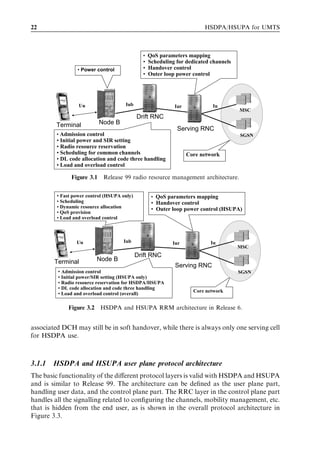
distribution is shown in Figure 3.1, and is covered in more detail in [1].
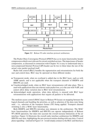
As scheduling has been moved to the BTS, there is now a change in the overall RRM
architecture. The SRNC will still retain control of handovers and is the one which will
decide the suitable mapping for quality of service (QoS) parameters. With HSDPA the
situation is simplified in the sense that as there are no soft handovers for HSDPA data,
then there is no need to run user data over multiple Iub and Iur interfaces and, even
though HSDPA is supported over Iur in the specifications, the utilization of the Iur
interface can be completely avoided by performing SRNC relocation, when the serving
high-speed downlink shared channel (HS-DSCH) cell is under a different controlling
RNC (CRNC). With Release 99 this cannot be avoided at RNC area boundaries when
soft handover is used between two base stations under different RNCs. Thus, the typical
HSDPA scenario could be presented by just showing a single RNC. Please note that the
HSDPA/HSUPA for UMTS: High Speed Radio Access for Mobile Communications Edited by Harri Holma
and Antti Toskala © 2006 John Wiley & Sons, Ltd. ISBN: 0-470-01884-4](https://image.slidesharecdn.com/wileyhsdpahsupaforumts-12712250730845-phpapp02/85/Hsdpa-Hsupa-For-Umts-38-320.jpg)
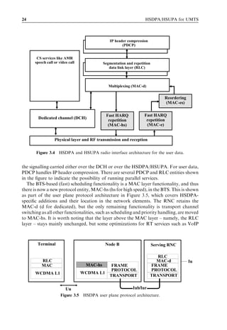
![HSPA architecture and protocols 25
Terminal Node B Serving RNC
RLC
RLC MAC-d
MAC MAC-es Iu
MAC-es/e MAC-e FRAME FRAME
PROTOCOL PROTOCOL
WCDMA L1 WCDMA L1
TRANSPORT TRANSPORT
Iub/Iur
Uu
Figure 3.6 HSUPA user plane protocol architecture.
were introduced for unacknowledged mode (UM) RLC in Release 6. As covered in the
introduction, even if HSDPA introduced physical layer retransmissions, there is still
the RLC layer handling the retransmissions should physical layer operation fail or,
especially, in connection with the different mobility events like serving HS-DSCH cell
change. This is assuming acknowledged mode (AM) RLC operation. In the case of
UM-RLC, physical year retransmissions are the only ones available. An example would
be a VoIP call where the RLC layer retransmissions from the RNC would be too slow.
With HSUPA there is in like manner a new MAC entity added to the BTS, as shown
in Figure 3.6. This is, however, not the only place where additions were made to the
protocol architecture. The terminal has a new MAC entity as well (MAC-es/s), to cover
the fact that part of the scheduling functionality is now moved to Node B, though it is
based on control information from the RNC and a direct capacity request from the user
equipment (UE) to the Node B. There is a new protocol entity for the RNC as well. This
is due to HSUPA soft handover and the fact that the physical layer retransmission
introduced in HSUPA has the effect of placing packets out of order. When data are
received in several BTS sites, there is a possibility when operating in the soft handover
region that packets from different BTSs arrive such that the order of packets is not
retained, and to allow reordering to be done for single packet streams the reordering
functionality needs to be combined with macro-diversity combining in MAC-es. Thus,
the new MAC-es ‘in-sequence delivery’ functionality has as its main task to ensure that
for the layers above the packets are provided in the order they were transmitted from the
terminal. Should such ordering be handled at the BTS, then an unnecessary delay would
be introduced as the BTS would have to wait for missing packets until they could be
determined to have been correctly received by another BTS in the active set. Further
details of the MAC layer architecture can be found in [2].
In like manner to HSDPA, the RLC layer in HSUPA is involved with the retransmis-
sion of packets if the physical layer fails to correctly deliver them after the maximum
number of retransmissions is exceeded or in connection with mobility events.
3.1.2 Impact of HSDPA and HSUPA on UTRAN interfaces
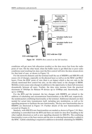
While the impacts of HSDPA and HSUPA in terms of data rates over the air interface are
well known and often the focus of discussion, the impact on the operation of the other
interfaces requires attention as well. For the interface between the base station and RNC,
the Iub interface, there are now larger data rates expected than with Release 99 terminals.](https://image.slidesharecdn.com/wileyhsdpahsupaforumts-12712250730845-phpapp02/85/Hsdpa-Hsupa-For-Umts-42-320.jpg)
![HSPA architecture and protocols 29
The terminal will now be able to accept multi-code transmission, which was the case in
Release 99 as well, but not implemented in the actual market place. Further details of
HSUPA-related new functionalities are covered in Chapter 5.
3.1.3 Protocol states with HSDPA and HSUPA
RRC states [1], [3] are the same with HSDPA and HSUPA as in Release 99. The
Cell_DCH is the state which is used when active data transmission to and from the
terminal on the DCH or HSDPA/HSUPA is possible. From Cell_DCH state the terminal
will be moved to Cell_FACH or further states, either directly from Cell_DCH state or via
Cell_FACH state if there are no data in the buffers. This happens depending on the
network timer settings after some seconds. There needs to be an obvious trade-off with
network response time for the first packet transmission instant after idle period and the
timer valve applied. The transitions take time due to the reconfiguration/setup processes
needed. Keeping a user booking HSDPA/HSUPA resource when there are no data to
transfer is not efficient from the system capacity or from the BTS resource use point of
view. Terminal battery life would also suffer, as keeping a terminal active with no data
passing through it will cause the battery to run out quickly.
Data can be transmitted in Cell_FACH state as well, but only using the forward access
channel (FACH) for the downlink and the random access channel (RACH) in the uplink,
which means limited data rates as these channels do not offer any of the performance
enhancement features of HSDPA and HSUPA. A terminal in Cell_FACH state con-
tinuously decodes FACH channels and then initiates the response downlink data (or
initiates transmission of data due in the uplink buffer) on the RACH. Depending on the
data volume (based on the reporting), the terminal may be moved back to Cell_DCH
state. As estimated in Chapter 10, the terminal battery power consumption ratio between
Cell_FACH state and Cell_DCH state is approximately 1 to 2, thus Cell_FACH state
should be avoided for lengthy time periods as well.
If the idle period in data transmission continues for lengthy periods, it makes sense to
move the terminal onwards to Cell_PCH or URA_PCH state. These states are the most
efficient ones from the terminal battery consumption point of view. Naturally, the use
of the discontinuous reception (DRX) cycle with the paging operation will cause some
additional delay to resume actual data transmission as the terminal needs to be paged
first. This happens in either one cell (location known at cell level in Cell_PCH state) or
in the registration area level (URA_PCH state). This is the benefit of the URA_PCH
state for terminals with high mobility. Terminals moving fast in a dense network would
necessitate a lot of cell updates, increasing the RACH load, but would then need to be
paged in multiple cells in case of downlink-originated activity. RRC states are illustrated
in Figure 3.11.
In idle mode there are no HSDPA/HSUPA-specific issues, the operation again uses the
DCH. Release 6 specifications indicate the position in the broadcast information at
which the network will inform whether there is HSUPA/HSDPA available, but this is
only for user information and not to influence the existing network and cell selection
behaviour. This has been defined in such a way in the specifications that early imple-
mentation (on top of Release 5) is possible as well. Obviously, the RRM reason will
dictate whether a user gets allocated HSDPA/HSUPA or not. Similarly to GPRS, it is](https://image.slidesharecdn.com/wileyhsdpahsupaforumts-12712250730845-phpapp02/85/Hsdpa-Hsupa-For-Umts-46-320.jpg)
![30 HSDPA/HSUPA for UMTS
DCH and/or Paging needed
HS-DSCH/E- for activity
DCH allocated
Connected mode
Cell DCH
Idle Cell PCH
mode
Cell FACH
URA PCH
FACH decoded
FACH decoded
continuosly
continuously
Figure 3.11 RRC states with HSDPA/HSUPA.
unknown before actual connection establishment how many slots – i.e., what practical
data rates – are available.
3.2 References
[1] H. Holma and A. Toskala (eds) (2004). WCDMA for UMTS (3rd edn). John Wiley & Sons.
[2] 3GPP, Technical Specification Group RAN: Medium Access Control (MAC) Protocol
Specification, 3GPP, TS 25.321, Version 6.7.0, Release 6. Available at www.3gpp.org
[3] 3GPP, Technical Specification Group RAN: Radio Resource Control (RRC) Protocol
Specification, 3GPP, TS 25.331, Version 6.8.0, Release 6. Available at www.3gpp.org](https://image.slidesharecdn.com/wileyhsdpahsupaforumts-12712250730845-phpapp02/85/Hsdpa-Hsupa-For-Umts-47-320.jpg)
![32 HSDPA/HSUPA for UMTS
actual implementation. For those interested in the historical reasons for DSCH use
please refer to [1] and the references therein for further details.
The FACH is used either for small data volumes or when setting up the connection and
during state transfers. In connection with HSDPA, the FACH is used to carry the
signalling when the terminal has moved, due to inactivity from Cell_DCH state to
Cell_FACH, Cell_PCH or URA_PCH state. The FACH is operated on its own and,
depending on the state the terminal is in, FACH is decoded either continuously
(Cell_FACH) or based on the paging message. For the FACH there is neither fast
power control nor soft handover. For the specific case of the Multimedia Broadcast
Multicast Service (MBMS), selection combining or soft combining may be used on the
FACH, but in any case there is no physical layer feedback for any activity on the FACH
and thus power control is not feasible. The FACH is carried on the secondary common
control physical channel (S-CCPCH) with fixed spreading factor. If there is a need for
service mix, like speech and data, then FACH cannot be used.
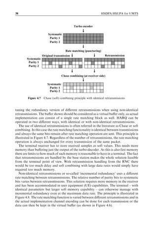
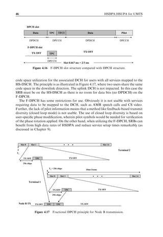
The Release 99 based DCH is the key part of the system – despite the introduction of
HSDPA – and Release 5 HSDPA is always operated with the DCH running in parallel
(as shown in Figure 4.1). If the service is only for packet data, then at least the signalling
radio bearer (SRB) is carried on the DCH. In case the service is circuit-switched – like
AMR speech call or video call parallel to PS data – then the service always runs on the
DCH. With Release 6 signalling can also be carried without the DCH, as explained in
connection with the fractional DCH (F-DCH). In Release 5, uplink user data always go
on the DCH (when HSDPA is active), whereas in Release 6 an alternative is provided by
the Enhanced DCH (E-DCH) with the introduction of high-speed uplink packet access
(HSUPA), as covered in Chapter 5.
The DCH can be used for any kind of service and it has fixed a spreading factor in the
downlink with fixed allocation during the connection. Thus, it reserves the code resources
corresponding to the peak data rate of the connection. Of course, higher layer signalling
could be used to reconfigure the code used for the DCH, but that is too slow to react to
changes in the traffic. In the case of multiple services, the reserved capacity is equal to the
sum of the peak data rate of the services. The theoretical peak rate is 2 Mbps but it seems
that 384 kbps is the highest implemented DCH data rate on the market so far. Any
HS
-S CC
H
HS
-DS
CH
HS
-DP
DC CC
H( H
DP
CC
H/D
PD
CH
Node B )
Terminal
Figure 4.1 Channels needed for HSDPA operation in Release 5.](https://image.slidesharecdn.com/wileyhsdpahsupaforumts-12712250730845-phpapp02/85/Hsdpa-Hsupa-For-Umts-49-320.jpg)
![HSDPA principles 33
Table 4.1 Comparison of fundamental properties of the DCH and HS-DSCH.
Feature DCH HS-DSCH
Variable spreading factor No No
Fast power control Yes No
Adaptive modulation and coding No Yes
Multi-code operation Yes Yes, extended
Physical layer retransmissions No Yes
BTS-based scheduling and link adaptation No Yes
scheduling and retransmission handling is done in the RNC. At the base station end, fast
power control is the key functionality for the DCH in addition to encoding the data
packet provided by the RNC. Soft handover (macro-diversity) is supported for the DCH,
and in such a case all base stations need to transmit exactly the same content (except for
power control commands) with identical timing to facilitate combining in the Rake
receiver.
HSDPA’s fundamental operation is based on the use of link adaptation, fast schedul-
ing and physical layer retransmission. All these methods have the aim of improving
downlink packet data performance both in terms of capacity and practical bit rates.
HSDPA does not support DCH features like fast power control or soft handover (as
summarized in Table 4.1).
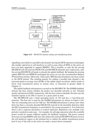
4.2 Key technologies with HSDPA
Several new channels have been introduced for HSDPA operation. For user data there
is the high-speed downlink shared channel (HS-DSCH) and the corresponding
physical channel. For the associated signalling needs there are two channels: high-
speed shared control channel (HS-SCCH) in the downlink and high-speed dedicated
physical control channel (HS-DPCCH) in the uplink direction. In addition to the basic
HSDPA channel covered in Release 5 specifications, there is now a new channel in
Release 6 specifications – the fractional dedicated physical channel (F-DPCH) – to cover
for operation when all downlink traffic is carried on the HS-DSCH. The channels needed
for HSDPA operation are shown in Figure 4.1. The channels missing from Figure 4.1 are
the broadcast channels from Release 99 for channel estimation, system information
broadcast, cell search, paging message transmission, etc., as covered in [1] in detail.
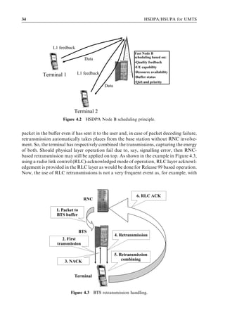
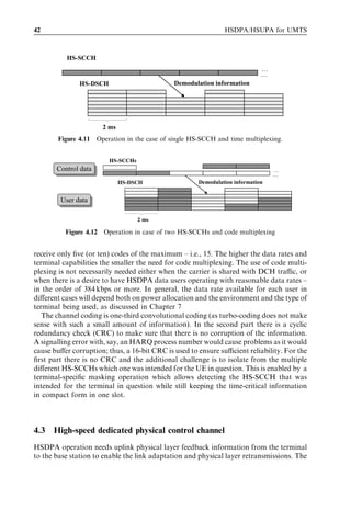
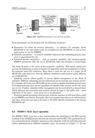
The general HSDPA operation principle is shown in Figure 4.2, where the Node B
estimates the channel quality of each active HSDPA user on the basis of the physical
layer feedback received in the uplink. Scheduling and link adaptation are then conducted
at a fast pace depending on the scheduling algorithm and the user prioritization scheme.
The other key new technology is physical layer retransmission. Whereas in Release 99
once data are not received correctly, there is a need for retransmission to be sent again
from the RNC. In Release 99 there is no difference in physical layer operation, regardless
of whether the packet is a retransmission or a new packet. With HSDPA the packet is
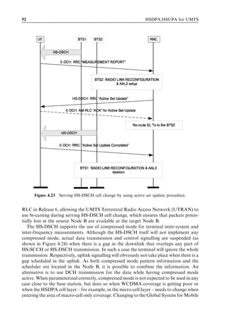
first received in the buffer in the BTS (as illustrated in Figure 4.3). The BTS keeps the](https://image.slidesharecdn.com/wileyhsdpahsupaforumts-12712250730845-phpapp02/85/Hsdpa-Hsupa-For-Umts-50-320.jpg)
![36 HSDPA/HSUPA for UMTS
Maximum rate
Data TPC TFCI Data Pilot
DPDCH DPCCH DPDCH DPCCH
Slot 0.667 ms = 2/3 ms
Reduced rate
Data TPC TFCI Data DTX Pilot
DPDCH DPCCH DPDCH DPCCH
Slot 0.667 ms = 2/3 ms
Figure 4.4 Discontinuous downlink transmission with Release 99 DCH.
down to, say, 16 kbps, the only way to reduce resource consumption would be to
reconfigure the radio link. This again takes time both when reconfiguring and ‘locking’
the data rate to a new smaller value until another reconfiguration would take place to
upgrade the data rate again. With the HS-PDSCH, once there are no data to be
transmitted, there is no transmission at all on the the HS-DSCH for the user in
question but the resource for the 2 ms is allocated to another user instead.
The HS-PDSCH is always transmitted on connection with the HS-SCCH and,
additionally, the terminal also always receives the DCH which carries services like
circuit-switched AMR speech or video as well as the SRB. Release 6 enhancements
enable operating with the SRB mapped on the HS-DSCH as well, as covered later
in connection with the section on the fractional dedicated physical channel (DPCH).
HS-PDSCH details are specified in [2].
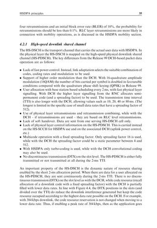
4.2.1.1 HS-DSCH coding
As covered in the introduction on the HS-DSCH, only turbo-coding is used for the
HS-DSCH. This was motivated by the fact that turbo-coding outperforms convolutional
coding otherwise expected with the very small data rates. The channel coding chain is
simplified from the corresponding DCH one, as there is no need to handle issues like
DTX or compressed mode with the HS-DSCH. Also, there is only one transport channel
active at a time, thus fewer steps in multiplexing/de-multiplexing are needed. An addi-
tional new issue is the handling of 16QAM and the resulting varying number of bits
carried by the physical channel even when the number of codes used remains fixed.
Another new functionality is bit scrambling on the physical layer for the HS-DSCH.
The HS-DSCH channel coding chain is illustrated in Figure 4.5.
For the 16QAM there is the specific function of constellation rearrangement, which
maps the bits to different symbols depending on the transmission numbers. This is
beneficial as with 16QAM all the symbols do not have equal error probability in the
constellation. This is due to different symbols having different numbers of ‘neighbouring’
symbols which places the symbols closer to the axis, with a greater number of neighbour-](https://image.slidesharecdn.com/wileyhsdpahsupaforumts-12712250730845-phpapp02/85/Hsdpa-Hsupa-For-Umts-53-320.jpg)
![HSDPA principles 39
Turbo encoder
Systematic
Parity 1
Parity 2
Rate matching (puncturing)
Original transmission Retransmission
Systematic
Parity 1
Parity 2
Incremental redundancy combining (at receiver side)
Systematic
Parity 1
Parity 2
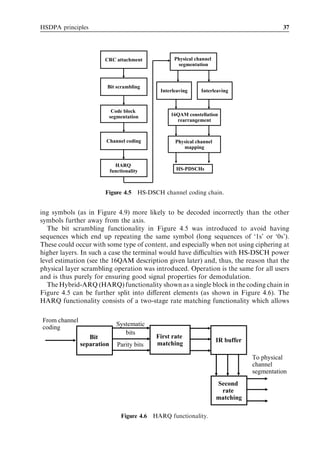
Figure 4.8 HARQ principle with non-identical retransmissions.
If physical layer retransmissions fail or exceed the maximum number of retransmis-
sions then the radio link layer (RLC) will handle further retransmissions. This typically
happens with serving HS-DSCH cell change or sometimes due to poor coverage or due to
a signalling error that could fill the buffer with undesired data. The latter rare event is due
to the error checks in the signalling, as covered in connection with the HS-SCCH details.
The physical channel segmentation in Figure 4.5 maps the data to physical channel
interleavers. The two interleavers are identical to Release 99 interleavers in the QPSK
case and in the 16QAM case when two interleavers are used. Note that as part of turbo-
coding there is a separate turbo-code internal interleaver in use. Details of the one-third
rate turbo-coder in use are unchanged from Release 99, based on the use of two parallel
concatenated convolutional code (PCCC) with two eight-state constituent encoders and
one turbo-code internal interleaver.
HS-DSCH channel coding is specified in Release 5 and in newer versions of [3].
4.2.1.2 HS-DSCH modulation
While the DCH only uses QPSK modulation, the HS-DSCH may additionally use the
higher order modulation: 16QAM. During the original HSDPA feasibility study other
alternatives – such as 8-PSK or 64QAM – were also discussed but not considered worth
adding to the system in addition to the link adaptation range already available with
QPSK and 16QAM and the different repetition/puncturing rates for turbo-coding. The
16QAM and QPSK constellations are shown in Figure 4.9. By having more constellation
points – 16 instead of 4 – now 4 bits can be carried per symbol instead of 2 bits per symbol
with QPSK.](https://image.slidesharecdn.com/wileyhsdpahsupaforumts-12712250730845-phpapp02/85/Hsdpa-Hsupa-For-Umts-56-320.jpg)
![40 HSDPA/HSUPA for UMTS
Minimum
constellation
point distance
QPSK 16QAM
Figure 4.9 QPSK and 16QAM constellations.
As shown in Figure 4.9, the use of higher order modulation introduces additional
decision boundaries. With 16QAM, it is no longer sufficient to not only have phase
figured out correctly but also amplitude needs to be estimated for more accurate phase
estimate. This explains why signal quality needs to be better when using 16QAM instead
of QPSK. In the downlink, a good-quality common pilot channel (CPICH) allows
estimation of the optimum channel without excessive user-specific pilot overhead.
The CPICH offers the phase information directly, but there is the need to estimate
the power difference between the CPICH and HS-DSCH power level to estimate the
amplitude information accurately as well. This suggests that at the base station end there
are also power changes that – during the 2-ms transmission – should be avoided.
The HS-DSCH can use a number of multicodes, with a spreading factor of 16. The
theoretical maximum number of codes available in a code tree with such a spreading
factor is 16, but as the common channels and associated DCHs need some room, the
maximum feasible number is 15. Whether a single terminal can receive up to 15 codes
during the 2-ms TTI depends on the terminal’s capabilities, as described in Section 4.5.
In the system there can be other traffic that are consuming code space as well – such as
CS speech or video calls – which cannot be mapped on HSDPA. Thus, radio resource
management will then determine the available code space for the scheduler at the BTS.
In principle, one could create more code space with secondary scrambling codes, but as
they are not orthogonal to the codes under the primary scrambling codes, the resulting
total capacity is not expected to increase. Thus, the use of other scrambling codes has
been restricted to compressed mode. HS-DSCH spreading and modulation is specified
in [4].
4.2.2 High-speed shared control channel
The HS-SCCH has two slots offset compared with the HS-DSCH (as shown in
Figure 4.10). This enables the HS-SCCH to carry time-critical signalling information
which allows the terminal to demodulate the correct codes. A spreading factor of 128
allows 40 bits per slot to be carried (with QPSK modulation). There are no pilots or
power control bits on the HS-SCCH and, thus, the phase reference is always the same as](https://image.slidesharecdn.com/wileyhsdpahsupaforumts-12712250730845-phpapp02/85/Hsdpa-Hsupa-For-Umts-57-320.jpg)
![HSDPA principles 47
As the SRBs are mapped to the HS-DSCH using the F-DPCH, the link quality from
the serving HS-DSCH cell is most critical. To ensure that there are appropriate criteria to
detect radio link failure, the terminal behaviour for setting the downlink power control
commands in the uplink DPCCH was modified so that the F-DPCH can be reliably
detected from the serving HS-DSCH cell. Thus, radio link failure is detected in the
terminal only from the F-DPCH of the serving HS-DSCH cell, and not from the soft
combined DPCCH as in Release 99.
4.3.2 HS-DSCH link adaptation
Link adaptation is very dynamic as it operates with 2-ms granularity with the HS-DSCH.
In addition to the scheduling decision, the MAC-hs in the BTS will also decide every 2 ms
which coding and modulation combination to transmit. Link adaptation is based on
physical layer CQI being provided by the terminal.
Using link adaptation, the network will also gain from the limitation of power control
dynamics in the downlink. As signals in the downlink cannot use too large a dynamic
range to avoid the near–far problem between signals from the same source, the downlink
power control dynamics is much more limited. While in the uplink a 71-dB or more
dynamic range is used, in the downlink only around 10 to 15 dBs can be utilized.
The exact number depends on the implementation, channel environment and spread-
ing factors applied. This means that for users close to the base station the power level
transmitted is higher than necessary for reliable signal detection. Link adaptation takes
this extra margin into use by selecting transmission parameters in such a way that the
required symbol energy corresponds more accurately to the available symbol power. This
is illustrated in Figure 4.18, where link adaptation as a function of the carrier-to-
interference ratio (C/I) is illustrated. As discussed previously, link adaptation itself is
based on CQI information that also takes other aspects into account besides just the
16 C/I received by
Instantaneous EsNo [dB]
C/I varies
Instantaneous Es/No [dB]
14 UE with fading
12
10
8
6
4
2
0
-2
0 20 40 60 80 100 120 140 160
Time [number of TTIs]
16QAM3/4 Link BTS adjusts link adaptation
adaptation mode with a few ms delay
16QAM2/4 mode based on channel quality
QPSK3/4 reports from the UE
QPSK2/4
QPSK1/4
Figure 4.18 Link adaptation.](https://image.slidesharecdn.com/wileyhsdpahsupaforumts-12712250730845-phpapp02/85/Hsdpa-Hsupa-For-Umts-64-320.jpg)
![HSDPA principles 49
4.3.2.1 HSDPA physical layer operation procedure
HSDPA physical layer operation goes through the following steps once one or more
users have been configured as using the HS-DSCH and data start to reach the buffer in
the Node B.
. The scheduler in the Node B evaluates – every 2 ms – for each user with data in the
buffer: the channel condition, buffer status, time from last transmission, retransmis-
sions pending and so forth. The exact criteria in the scheduler are naturally a vendor-
specific implementation issue and not part of 3GPP specifications. Parameters to
control scheduler behaviour have been specified and are covered in Section 4.5.2.
. Once a terminal has been determined as serving in a particular TTI, the Node B
identifies the necessary HS-DSCH parameters, including number of codes, 16QAM
usability and terminal capability limitations.
. The Node B starts to transmit the HS-SCCH two slots before the corresponding HS-
DSCH TTI. HS-SCCH selection is free (from a set of at most four channels) assuming
there were no data for the terminal in the previous HS-DSCH frame. Had there been
data in the previous frame, then the same HS-SCCH needs to be used.
. The terminal monitors the terminal-specific set of at most four HS-SCCHs given by the
network. Once the terminal has decoded Part 1 from an HS-SCCH intended for that
terminal, it will start to decode the remaining parts of that HS-SCCH and will buffer
the necessary codes from the HS-DSCH.
. After decoding the HS-SCCH parameters from Part 2, the terminal can determine to
which ARQ process the data belong and whether they need to be combined with data
already in the soft buffer.
. In the Release 6 version, a pre-amble is sent in the ACK/NACK field if the feature is
configured to be used by the network (and if there was no packet in the previous TTI).
Sending of the pre-amble is based on HS-SCCH decoding, not on the HS-DSCH itself.
. Upon decoding the potentially combined data, the terminal sends in the uplink
direction an ACK/NACK indicator, depending on the outcome of the CRC conducted
on the HS-DSCH data (an ACK follows the correct CRC outcome).
. If the network continues to transmit data for the same terminal in consecutive TTIs,
the terminal will stay on the same HS-SCCH that was used during the previous TTI.
. In Release 6, when the data flows end, the terminal sends a post-amble in the ACK/
NACK field, assuming the feature was activated, of course.
HSDPA operation is synchronous in terms of the terminal response for a packet
transmitted in the downlink. The network side, however, is asynchronous in terms of
when a packet or a retransmission for an earlier transmission is sent. This allows the
necessary freedom for BTS scheduler implementation and is enabled by ARQ process
information on the HS-SCCH. The physical layer operation procedure for HSDPA is
covered in [5].
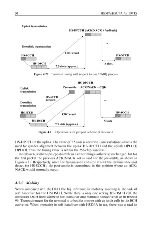
The terminal operation times between different events are specified accurately from the
HS-SCCH reception, followed by HS-DSCH decoding and ending with the uplink ACK/
NACK transmission. As indicated in Figure 4.20, there is a 7.5-slot reaction time from
the end of the HS-DSCH TTI to the start of ACK/NACK transmission in the](https://image.slidesharecdn.com/wileyhsdpahsupaforumts-12712250730845-phpapp02/85/Hsdpa-Hsupa-For-Umts-66-320.jpg)
![HSDPA principles 53
DL DCH for Terminal 1
HS-SCCH Compressed frame
…
HS-DSCH
…
2 ms Not permitted HS-DSCH TTI for Terminal 1
Figure 4.24 HSDPA operation with compressed mode.
Communications (GSM) obviously causes a drop in the user data rate, the actual
difference depending on GSM network capabilities. The available data rate varies theo-
retically up to 384 kbps depending whether there is only a basic (GPRS) service available
or whether the enhanced data rate for global evolution (EDGE) is also supported. The
channel conditions and number of slots supported in the multimode terminal limit the
practical data rates to around 200 to 300 kbps (as discussed in Chapter 10).
For the handover to/from GSM networks, the Release 6 specifications contain support
for packet handover. This allows reducing the handover interruption time to similar level
achieved by Release 99 based voice call handovers, where the end user in a properly
parameterized network does not detect the change of system. In Release 5 there is
network-assisted cell change when changing to GSM to speed up the process, while
in Release 99 based networks only cell reselection from WCDMA is available to GSM.
4.4 BTS measurements for HSDPA operation
There are three new BTS measurements specified in Release 5 that facilitate receipt of the
necessary information about HSDPA operation in the RNC. In the physical layer there is
the following measurement (defined in [6]):
. Non-HSPDA power, which basically reveals the power being used for all channels
other than HSDPA (HS-DSCH and HS-SCCH). In the Release 6 version this meas-
urement covers all downlink channels not used for HSDPA or HSUPA purposes.
There is no point in measuring actual HSDPA power as that is either the difference
between non-HSDPA power and the maximum BTS transmission power, or HSDPA
power allocation has been provided by the RNC.
It is in the scheduler – this part of the MAC layer is covered in [7] – that the HS-DSCH
provides a bit rate measurement. This measurement gives information on the average
data rate per each priority class over the measurement period.](https://image.slidesharecdn.com/wileyhsdpahsupaforumts-12712250730845-phpapp02/85/Hsdpa-Hsupa-For-Umts-70-320.jpg)
![54 HSDPA/HSUPA for UMTS
Further, a common measurement in Iub [8] is definition of the required power for the
HS-DSCH. This gives information about the estimated power per priority class required
to meet the guaranteed bit rate value. Additionally, the Node B could list the terminals
which require very high power for meeting their guaranteed bit rate for connection.
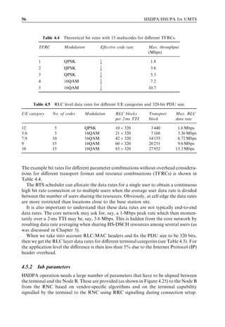
4.5 Terminal capabilities
Support of the HSDPA feature itself is optional for terminals. When supporting HSDPA
operation, the terminal will indicate one of the 12 different categories specified. Depend-
ing on the category supported, the resulting maximum downlink data rates vary between
0.9 and 14.4 Mbps. HSDPA capability is otherwise independent of Release 99 based
capabilities, but if the HS-DSCH has been configured for the terminal, then DCH
capability in the downlink is limited to the value given by the terminal. A terminal
can indicate a 32, 64, 128 or 384-kbps DCH capability; thus, a terminal normally capable
of running at 384 kbps on the DCH may indicate that – once HSDPA is configured – the
DCH should be reconfigured down to 64 kbps.
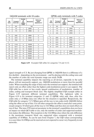
The first ten HSDPA terminal capability categories in Table 4.2 need to support
16QAM, but the last two, categories 11 and 12, only support QPSK modulation. The
other key difference between the classes is the maximum number of parallel codes that
must be supported. Another value indicating the capability to sustain the peak rate over
multiple continuous TTIs is the inter-TTI parameter. Categories with a value of 1
correspond to devices that can also sustain the peak rate during 2 ms over multiple
TTIs, while terminals with an inter-TTI value greater than 1 must ‘rest’ for 2 or 4 ms after
each received TTI. Additionally, there is a soft buffer capability which uses two principles
for determining its value.
Table 4.2 HSDPA terminal capability categories.
Category Maximum Minimum Transport ARQ type at Achievable
number of inter-TTI channel bits maximum maximum
parallel codes interval per TTI data rate data rate
per HS-DSCH (Mbps)
1 5 3 7 298 Soft 1.2
2 5 3 7 298 IR 1.2
3 5 2 7 298 Soft 1.8
4 5 2 7 298 IR 1.8
5 5 1 7 298 Soft 3.6
6 5 1 7 298 IR 3.6
7 10 1 14 411 Soft 7.2
8 10 1 14 411 IR 7.2
9 15 1 20 251 Soft 10.2
10 15 1 27 952 IR 14.4
11 5 2 3 630 Soft 0.9
12 5 1 3 630 Soft 1.8](https://image.slidesharecdn.com/wileyhsdpahsupaforumts-12712250730845-phpapp02/85/Hsdpa-Hsupa-For-Umts-71-320.jpg)
![HSDPA principles 55
Table 4.3 RLC parameters for different UE categories.
UE category Maximum number Minimum total RLC AM
AM RLC entities and MAC-hs memory
1–6, 11 and 12 6 50 kbytes
7–8 8 100 kbytes
9–10 8 150 kbytes
AM ¼ acknowledged mode.
Terminals with a smaller soft buffer value – for example, category 5 – cannot deal with
incremental redundancy at the higher data rates (closer to the 3.6-Mbps peak rate), so the
network has to use soft/chase combining instead. Whether this is the case depends also on
the total number of ARQ processes configured and on relative memory partitioning.
The highest capability is provided with category 10, which allows the theoretical
maximum data rate of 14.4 Mbps. This rate is achievable with one-third rate turbo-
coding and significant puncturing resulting in a code rate close to 1 – that is, hardly any
coding. For category 9, the maximum turbo-encoding block size (from Release 99) has
been taken into account when calculating the values, and thus results in the 10.2-Mbps
maximum user data rate value with four turbo-encoding blocks.
Besides the physical category to be reported to the network there are other parameters
important for HSDPA operation. The size of the RLC reordering buffer determines the
window length of the packets that can be ‘in the pipeline’ to ensure in-sequence delivery
of data to higher layers in the terminal. The minimum values range from 50 to 150 kB
depending on the UE category (as can be seen from Table 4.3). The buffer size has been
derived so that there should be no limitations to the data rate due to this, assuming
UTRAN end delays (including RLC retransmission handling) are reasonable and, thus,
the memory needed for the RLC buffer does not get too large.
There is a link in the terminal capability with Release 6 HSUPA. The support of
HSDPA is mandatory for a terminal that supports high-speed uplink packet access
(HSUPA) in Release 6, but the HSDPA category can be chosen freely. Release 6 HSDPA
additions – like F-DPCH or the pre/post scheme – are mandatory for Release 6 HSDPA
capable terminals, while support for features like advanced receivers or receiver antenna
diversity depends on a particular implementation and is not part of terminal capability
signalling. The terminal capabilities for HSDPA operation are specified in [9].
4.5.1 L1 and RLC throughputs
The physical layer data rate is constructed from the following parameters:
. number of codes in use;
. modulation;
. effective coding rate – that is, the amount of repetition or puncturing on top of the
turbo-encoder output.](https://image.slidesharecdn.com/wileyhsdpahsupaforumts-12712250730845-phpapp02/85/Hsdpa-Hsupa-For-Umts-72-320.jpg)
![HSDPA principles 59
DTCHs
Multiplexing (MAC-d in RNC)
MAC-d flow
MAC-hs in BTS
HS-DSCH
Physical layer HS-DSCH
HS-PDSCH
Figure 4.27 MAC-d multiplexing of logical channels into a single MAC-d flow.
separate MAC-d header is added; otherwise, there is no need to have a MAC-d header
with HSDPA and, thus, no actual operation takes place in MAC-d.
There are two logical channels relevant for HSDPA operation. These channels are
mapped in the MAC layer to transport channels and then further in the physical layer to
physical channels. The dedicated traffic channel (DTCH) carries user data, while the
dedicated control channel (DCCH) carries the control information – like RRC signal-
ling. The DCCH cannot be mapped to the MAC-d flow in Release 5, but in Release 6 the
additional functionality is defined to ensure proper terminal behaviour just in case the
connection to the serving HS-DSCH cell is lost. HSPDA MAC layer operation is
specified in [7].
DTCH with PS
domain service
HS
-DS
CH
DC
H
Node B
Terminal
DCCH & DTCH with CS
or PS domain service
Figure 4.28 Logical channel mapping with Release 5 HSDPA.](https://image.slidesharecdn.com/wileyhsdpahsupaforumts-12712250730845-phpapp02/85/Hsdpa-Hsupa-For-Umts-76-320.jpg)
![60 HSDPA/HSUPA for UMTS
Also, the earlier described F-DPCH enables benefiting from reduced code resource
needs if there are no services requiring a Release 99 type DCH to be allocated. For the
DTCH, allocation depends on the type of service in question. For the circuit-switched
(CS) domain service, obviously the DCH is always to be used (as shown in Figure 4.28),
while for packet-switched (PS) domain allocation the choice is influenced by several
service parameters as well as the radio resource situation.
The properties of the scheduler have an impact on what kind of service should be
carried on HS-DSCH. Also if the delay requirements are very tight, there is less gain in
having those allocated on HSDPA as there is not much the scheduler can do. The
HSDPA radio resource management issues are covered in Chapter 6.
4.7 References
[1] H. Holma and A. Toskala (eds) (2004), WCDMA for UMTS (3rd edn), John Wiley & Sons,
Chichester, UK.
[2] 3GPP, Technical Specification Group RAN, Physical channels and mapping of transport
channels onto physical channels (FDD), 3GPP TS 25.211 version 6.7.0, Release 6, available
at www.3gpp.org
[3] 3GPP, Technical Specification Group RAN, Multiplexing and channel coding (FDD),
3GPP TS 25.212 version 6.7.0, Release 6, available at www.3gpp.org
[4] 3GPP, Technical Specification Group RAN, Spreading and modulation (FDD), 3GPP TS
25.213 version 6.4.0, Release 6, available at www.3gpp.org
[5] 3GPP, Technical Specification Group RAN, Physical layer procedures (FDD), 3GPP TS
25.214 version 6.7.1, Release 6, available at www.3gpp.org
[6] 3GPP, Technical Specification Group RAN, Physical layer – measurements (FDD), 3GPP
TS 25.215 version 6.4.0, Release 6, available at www.3gpp.org
[7] 3GPP, Technical Specification Group RAN, Medium Access Control (MAC) protocol
specification, 3GPP TS 25.321 version 6.7.0, Release 6, available at www.3gpp.org
[8] 3GPP, Technical Specification Group RAN, Iub, 3GPP TS 25.433 version 6.8.0, Release 6,
available at www.3gpp.org
[9] 3GPP, Technical Specification Group RAN, UE radio access capabilities definition, 3GPP
TS 25.306 version 6.7.0, Release 6, available at www.3gpp.org](https://image.slidesharecdn.com/wileyhsdpahsupaforumts-12712250730845-phpapp02/85/Hsdpa-Hsupa-For-Umts-77-320.jpg)
![62 HSDPA/HSUPA for UMTS
Data + Feedback (L1/MAC)
Fast Node B uplink
scheduling control
based on:
Scheduler control •Resource feedback
•UE capability
Data + Feedback
Terminal 1 •Resource availability
•Terminal buffer status
•QoS and Priority
Scheduler control
Terminal 2
Figure 5.1 HSUPA Node B (BTS) scheduling principle.
the basic power control loop functions in Release 99 are just as essential for HSUPA
operation.
HSUPA provides a flexible path beyond the 384-kbps uplink which can be seen as the
realistic maximum for WCDMA before HSUPA. A similar technology to that of
HSDPA is being used by introducing fast uplink hybrid-ARQ (HARQ), Node B
based uplink scheduling (as shown in Figure 5.1) and easier multicode transmission
than with Release 99.
The focus in this chapter is on the additions to the Release 6 specifications that the
HSUPA feature entails, and the functionality of the Release 99 uplink is described as a
reference in the most relevant cases. Anyway, it is worth keeping in mind that none of the
old features were replaced by HSUPA and that it was more of an add-on than a
replacement. The complete description of all the features needed for, say, synchroniza-
tion and cell search can be found in [1].
5.2 Key technologies with HSUPA
5.2.1 Introduction
The HSUPA feature of the 3GPP WCDMA system is in fact a new uplink transport
channel – E-DCH – that brought some of the same features to the uplink as the HSDPA
with its new transport channel – high-speed downlink shared channel (HS-DSCH) –
provided for the downlink. The E-DCH transport channel supports fast Node B based
scheduling, fast physical layer HARQ with incremental redundancy and, optionally, a
shorter 2-ms transmission time interval (TTI). Though – unlike HSDPA – HSUPA is not
a shared channel, but a dedicated one, by structure the E-DCH is more like the DCH of
Release 99 but with fast scheduling and HARQ than an uplink HSDPA: that is, each UE
has its own dedicated E-DCH data path to the Node B that is continuous and inde-
pendent from the DCHs and E-DCHs of other UEs. Table 5.1 lists the applicability of
the key features for DCH, HSDPA and HSUPA.](https://image.slidesharecdn.com/wileyhsdpahsupaforumts-12712250730845-phpapp02/85/Hsdpa-Hsupa-For-Umts-79-320.jpg)
![HSUPA principles 63
Table 5.1 HSDPA, HSUPA and DCH comparison table.
Feature DCH HSDPA (HS-DSCH) HSUPA (E-DCH)
Variable spreading factor Yes No Yes
Fast power control Yes No Yes
Adaptive modulation No Yes No
BTS based scheduling No Yes Yes
Fast L1 HARQ No Yes Yes
Soft handover Yes No Yes
TTI length [ms] 80, 40, 20, 10 2 10, 2
Respectively, new signalling channels are needed (as shown in Figure 5.2); all the
channels (excluding broadcast ones) shown in the figure are necessary for HSUPA
operation. In Figure 5.2 it is assumed that downlink is on the DCH while in most
cases it is foreseen that HSDPA could be used, but for clarity only the downlink DCH is
shown in addition to HSUPA-related channels.
The channels for scheduling control – E-DCH absolute grant channel (E-AGCH) and
E-DCH relative grant channel (E-RGCH) – as well as retransmission support on the
E-DCH HARQ indicator channel (E-HICH) are covered in detail in later sections. The
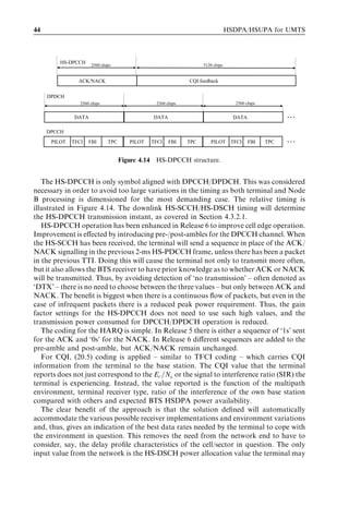
user data is carried on the enhanced dedicated physical data channel (E-DPDCH) while
new control information is on the E-DPCCH, as will be covered in later sections. From
the Release 99 DCH, the dedicated physical control channel (DPCCH) is unchanged and
the need for the DPDCH depends on possible uplink services mapped to the DCH.
Unlike HSDPA, HSUPA does not support adaptive modulation because it does not
support any higher order modulation schemes. This is due to the fact that more complex
modulation schemes require more energy per bit to be transmitted than simply going for
transmission with multiple parallel code channels using simple binary phase shift keying
(BPSK) modulation.
In the downlink – due to the smaller dynamic range of transmitted channel power –
there are cases where the downlink signal is transmitted in any case with more energy
E -H
IC
H/E
-R G
CH
E-A
GC
H
E-D
P CC
H
E-D
PD
CH
DC
H (D P
CC
Node B H /DP
DC
H) Terminal
Figure 5.2 Channels needed for HSUPA operation when downlink is on the Release 99 DCH.](https://image.slidesharecdn.com/wileyhsdpahsupaforumts-12712250730845-phpapp02/85/Hsdpa-Hsupa-For-Umts-80-320.jpg)
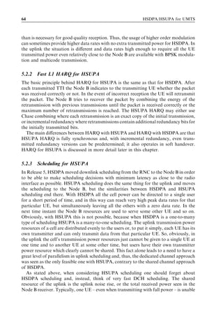
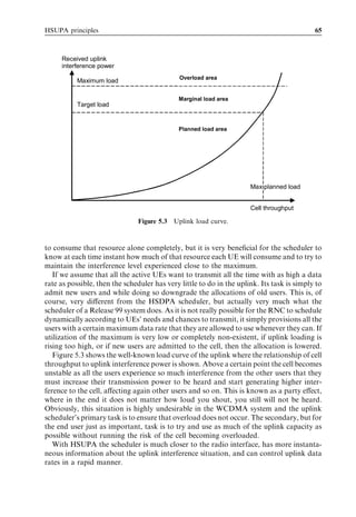
![66 HSDPA/HSUPA for UMTS
5.3 E-DCH transport channel and physical channels
5.3.1 Introduction
As said in previous chapters, HSUPA is a new uplink transport channel, E-DCH, which
supports enhanced features to those of the uplink transport channels of Release 99.
Uplink transport channel processing for E-DCH is similar to the processing of the uplink
DCH with two exceptions. There can be only one E-DCH transport channel in the UE as
there may be multiple parallel DCHs that are multiplexed together to a single coded
composite transport channel (CCTrCH) of DCH type. Nevertheless, the MAC layer can
multiplex multiple parallel services to the single E-DCH. The other significant difference
is HARQ support for the E-DCH which is provided in the transport channel processing
chain and is, of course, something totally new.
After transport channel processing, the E-DCH maps to one or multiple parallel new
dedicated physical data channels – E-DPDCHs – for physical layer transmission. This
is completely parallel to uplink DCH processing chain and physical channels, so both
E-DCH and DCH can coexist in the same UE with the restriction that the maximum
DCH data rate is 64 kbps when the E-DCH is configured.
Using E-DPDCH transmissions a simultaneous and parallel control channel is sent a
separate code channel – E-DPCCH. This E-DPCCH transmits all the necessary informa-
tion about the E-DPDCH that is needed in order to know how to receive the data
channel.
In the downlink three new physical channels were introduced to provide HARQ
feedback and facilitate uplink scheduling. The E-DCH HARQ indicator channel (E-
HICH) sends the HARQ acknowledgement information back to the UE. The E-RGCH
provides relative step-up/down scheduling commands and the E-AGCH provides an
absolute scheduling value for the UE. All the new physical channels are described in
detail in [2] and covered in the following sections.
5.3.2 E-DCH transport channel processing
Transport channel processing is the functionality that transforms the transport blocks
delivered by the MAC layer to bits transmitted on physical channels. Figure 5.4 shows
the overview of DCH and E-DCH transport channel processing from the MAC layer to
the physical channels. Transport channel processing for both the DCH and E-DCH are
described in detail in [3].
A single E-DCH transport channel processing chain always gets one transport block
to process for transmission in one TTI, because – for the DCH – a set of transport blocks
for each configured DCH will be delivered to the processing chain. In Figure 5.5 the
differences between the elements of transport channel processing chains for the E-DCH
and DCH are illustrated:
. CRC attachment for the E-DCH always attaches a 24-bit CRC to the transport block
received from the MAC layer. In comparison, the CRC length for the DCH is
configurable and can be 0, 8, 12, 16, or 24 bits.](https://image.slidesharecdn.com/wileyhsdpahsupaforumts-12712250730845-phpapp02/85/Hsdpa-Hsupa-For-Umts-83-320.jpg)
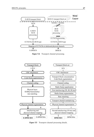
![68 HSDPA/HSUPA for UMTS
. Code block segmentation for the E-DCH splits its input into equal size code blocks so
that the length of the block does not exceed 5114 bits. For the DCH the same block first
concatenates the transport block set to a single block of data before splitting. Also the
size of the maximum code block with the DCH depends on the coding in use (5114 for
turbo-coding and 504 for convolutional coding).
. Channel coding for the E-DCH is always turbo-coding with a code rate of 1/3. DCH
channel coding may be either convolutional coding with code rates 1/2 or 1/3 or turbo-
coding with a code rate of 1/3.
. Physical layer HARQ funtionality/rate matching for the E-DCH matches the channel
codes output bits to the available physical channel bits and produces the different
redundancy versions needed for incremental redundancy HARQ.
. Physical channel segmentation for the E-DCH distributes the channel bits among the
multiple E-DPDCHs if more than one E-DPDCH is needed. The functionality is also
the same in the corresponding block in the DCH processing chain.
. Interleaving and physical channel mapping for the E-DCH, as well as for the DCH,
interleaves the bits in the radio frame and maps the bits to be transmitted to their final
positions in the physical channel.
5.3.3 E-DCH dedicated physical data channel
The E-DPDCH is a new uplink physical channel used for transmitting bits – as a result of
E-DCH transport channel processing – from the mobile to the base station. It is a new
channel that exists parallel to all the uplink dedicated channels of the 3GPP Release 5
(DPDCH and DPCCH used for uplink data transmission and HS-DPCCH used for
HSDPA feedback delivery). Thus, with the introduction of HSUPA there may be up to
five different types of dedicated channels transmitted simultaneously in the uplink.
The E-DPDCH has a very similar structure to the DPDCH of Release 99 with a few
exceptions. They both support orthogonal variable spreading factors (OVSFs) to adjust
the number of channel bits to the amount of data actually being transmitted. They both
could go beyond the data rate that one physical data channel can support by transmitting
multiple channels in parallel [4]. They both use BPSK modulation and follow the same
fast power control loop.
The most notable properties of the E-DPDCH that the DPDCH does not have are the
ones that make HSUPA what it is: the E-DPDCH supports fast physical layer level
HARQ and fast Node B based scheduling. However, these are not really properties of the
physical data channel as such, but the HARQ is visible in the transport channel
processing chain and the scheduling is visible in the MAC layer. The differences in
the actual physical data channels are a bit more subtle.
The biggest difference for E-DPDCH is the support of a spreading factor (SF) of 2,
which allows delivering twice as many channel bits per code than the minimum spreading
factor of 4 that the DPDCH supports. However, this is not the whole truth as the
DPDCH could support six parallel SF4 codes as the E-DPDCH supports simultaneous
transmission of two SF2 and two SF4 codes which both lead to the maximum physical
layer bit rate of 5.76 Mbps.
The steps for supporting the data rates is different. Both DPDCH and E-DPDCH
support spreading factors 256, 128, 64, 32, 16, 8, and 4 and respective physical channel](https://image.slidesharecdn.com/wileyhsdpahsupaforumts-12712250730845-phpapp02/85/Hsdpa-Hsupa-For-Umts-85-320.jpg)
![HSUPA principles 69
Table 5.2 Physical channel bit rate steps for DPDCH and E-DPDCH.
Channel bit rates DPDCH E-DPDCH
15–960 kbps SF256–SF4 SF256–SF4
1.92 Mbps 2 Â SF4 1 2 Â SF4
2880 Mbps 3 Â SF4 1 —
3840 Mbps 4 Â SF4 1 2 Â SF2
4800 Mbps 5 Â SF4 1 —
5760 Mbps 6 Â SF4 1 2 Â SF4 þ 2 Â SF2
1
Multicode not supported in practice with DPDCH.
bit rates of 15, 20, 60, 120, 240, 480, and 960 kpbs with a single OVSF code transmission.
If the 960-kbps channel bit rate provided by spreading factor 4 is insufficient to transmit
all the data from transport channel processing, then both move to using two SF4 codes in
parallel and achieve a 1920-kpbs physical channel bit rate. Things only go differently for
the two types of dedicated data channels beyond this point. After two parallel SF4 codes
the DPDCH has steps for three, four, five, and six parallel SF4 codes up to a 5.76-Mbps
channel bit rate. The E-DPDCH has fewer steps and uses a spreading factor of 2. After
two SF4 codes, the E-DPDCH goes directly to two SF2 codes. These steps are shown
in Table 5.2. Usage of two SF2 codes provides some gains over using three or four
parallel SF4 codes for the transmitter’s peak to average power ratio and enables
implementing a more power-efficient amplifier for UEs supporting very high data
rate transmission.
The most notable physical layer difference between the two data channels is the new
TTI length of 2 ms supported by the E-DPDCH. This is achieved by maintaining the
10-ms radio frame structure already familiar with the DPDCH, but when a 2-ms TTI is in
use the 10-ms radio frame is divided into five independent sub-frames. The differences
between the DPDCH and E-DPDCH are listed in Table 5.3. Table 5.4 shows the physical
channel data rates for different spreading factors for both the DPDCH and E-DPDCH.
Table 5.3 DPDCH and E-DPDCH comparison table.
Feature DPDCH E-DPDCH
Maximum SF 256 256
Minimum channel data rate 15 kbps 15 kbps
Minimum SF 4 2
Maximum channel data rate 960 kbps 1920 kbps
Fast power control Yes Yes
Modulation BPSK BPSK
Soft handover Yes Yes
TTI length [ms] 80, 40, 20, 10 10, 2
Maximum no. of parallel codes 6 Â SF4 1 2 Â SF2 þ 2 Â SF4
1
Practical maximum for DPDCH is 1 Â SF4.](https://image.slidesharecdn.com/wileyhsdpahsupaforumts-12712250730845-phpapp02/85/Hsdpa-Hsupa-For-Umts-86-320.jpg)
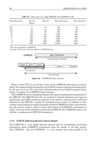
![HSUPA principles 71
Table 5.5 Slot format of E-DPCCH.
Spreading factor Bit rate Bits/slot Bits/radio frame Bits/sub-frame
(kbps)
256 15 10 150 30
uplink dedicated channels of 3GPP Release 5, and always accompanies E-DPDCH
transmission.
To some extent the E-DPCCH does the same for E-DPDCH transmission as the
DPCCH does for DPDCH transmission – that is, the control channel delivers the
information needed to decode the corresponding data channel transmission. The
principal difference between the two is that – in addition to information about the
DPDCH – the DPCCH also provides common information related to, for example,
channel estimation and power control, while the E-DPDCH only contains information
about the E-DPDCH.
The E-DPCCH has only one possible slot format (as shown in Table 5.5), which uses
a spreading factor of 256 and is capable of delivering 30 channel bits in a 2-ms sub-frame.
It is designed to deliver 10 bits of information for each E-DPDCH TTI transmitted. The
E-DPCCH uses the same (30, 10) second-order Reed–Muller coding as used for transport
format combination indicator (TFCI) coding in the DPCCH. This means that the 10
information bits result in 30 bits to be transmitted in the physical channel. This number
of bits can be carried by the E-DPCCH in 2 ms. If the TTI length of the E-DPDCH is
10 ms, then the 30-bit E-DPCCH sub-frame is repeated five times allowing reduced
power level. With this procedure the same E-DPCCH structure can be employed
regardless of the TTI used for E-DPDCH transmission. The E-DPCCH frame structure
is illustrated in Figure 5.7 and the coding and mapping of E-DPCCH bits are described in
detail in [3].
The 10 information bits on the E-DPCCH consist of three different segments:
. E-TFCI, the E-DCH transport format combination indicator of 7 bits indicating
the transport format being transmitted simultaneously on E-DPDCHs. In essence,
the E-TFCI tells the receiver the transport block size coded on the E-DPDCH. From
this information the receiver can derive how many E-DPDCHs are transmitted in
parallel and what spreading factor is used.
Data: 10 info bits coded to 30 channel bits E-DPCCH
3 slots, 7680 chips
Slot#0 Slot#1 Slot#2
Slot#i Slot#14
2 ms sub-frame
10ms radio frame
Figure 5.7 E-DPCCH frame structure.](https://image.slidesharecdn.com/wileyhsdpahsupaforumts-12712250730845-phpapp02/85/Hsdpa-Hsupa-For-Umts-88-320.jpg)
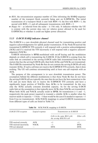
![HSUPA principles 73
1-bit of information E-HICH/E-RGCH
3 slot, 7680 chips, 120 channel bits
40-bit long signature sequence
1 slot, 2560 chips, 40 bits
Slot#0 Slot#1 Slot#2
Slot#i Slot#14
2 ms sub-frame
10ms radio frame
Figure 5.8 E-HICH/E-RGCH frame structure.
All the cells in the same Node B are assumed to receive uplink E-DPDCH transmission
in cooperation and, thus, even if there are multiple cells in the Node B participating in a
softer handover the TTI reception either succeeds or fails only once, not separately in
all the cells. Due to this all E-HICHs transmitted from the Node B containing the serving
E-DCH cell transmit both ACKs and NACKs, effectively enabling the UE to combine
the radio links for more reliable ACK/NACK detection.
E-HICH and E-RGCH channel structures are exactly the same, and they are illus-
trated in Figure 5.8. Each delivers 1 bit of information in three slots. In the case of a
10-ms TTI the three slots are repeated four times resulting in an 8-ms-long message.
The exception is the E-RGCH transmitted from cells not belonging to the serving
E-DCH radio link set. That channel always – regardless of the E-DCH TTI – transmits
a 10-ms-long message (i.e., the three slots are always repeated five times).
The E-HICH/E-RGCH basic building block is a 40-bit-long orthogonal sequence
which allows the orthogonal multiplexing of 40 bits in one slot on a single spreading
factor 128-code channel. The same E-HICH/E-RGCH bit is repeated three times over
three slots, but uses a different signature in each of the three slots following a deter-
ministic code hopping pattern. This is because different signature pairs have different
isolations in a real radio environment and, thus, the effect is averaged this way. Signature
sequences and hopping patterns are defined in [2].
E-HICHs and E-RGCHs utilize 40-bit-long orthogonal sequences for multiplexing
multiple E-HICHs and E-RGCHs (40 in total) to a single downlink code channel of
spreading factor 128.
One cell can use multiple channelization codes to exceed the limit of 40 signatures
(e.g., 20 E-HICHs and 20 E-RGCHs in a code) with the constraint that the E-HICH and
E-RGCH intended for the same UE must be transmitted with the same channelization
code. Figure 5.9 illustrates the Node B operation for combining up to 40 signatures on a
single downlink channelization code.
5.3.6 E-DCH relative grant channel
The E-RGCH is a new downlink physical channel used for transmitting single step-up/
down scheduling commands that affect the relative transmission power the UE is allowed](https://image.slidesharecdn.com/wileyhsdpahsupaforumts-12712250730845-phpapp02/85/Hsdpa-Hsupa-For-Umts-90-320.jpg)
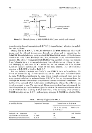
![HSUPA principles 75
As mentioned above, E-RGCH frame structure and signature generation is exactly
the same as for the E-HICH (Figures 5.8 and 5.9). Differentiation is in the higher layers –
that is, the network informs the UE by means of RRC signalling that signature x on
channelization code k is the E-HICH and signature y on the same channelization code
is the E-RGCH.
5.3.7 E-DCH absolute grant channel
The E-AGCH is a new downlink physical channel used for transmitting an absolute
value of the Node B scheduler’s decision that lets the UE know the relative transmission
power it is allowed to use for data channel transmission (E-DPDCH), thus effectively
telling the UE the maximum transmission data rate it may use.
The E-AGCH delivers 5 bits to the UE for the absolute grant value, indicating the
exact power level the E-DPDCH may use in relation to the DPCCH. In addition, the E-
AGCH carries a 1-bit indication for the absolute grant scope. With this bit the Node B
scheduler can allow/disallow UE transmission in a particular HARQ process. This bit is
only applicable for 2-ms TTI E-DCH operation. In addition to this the E-AGCH uses a
primary and a secondary UE-id for identifying the intended receiver and delivering one
additional bit of information. The E-AGCH coding chain is illustrated in Figure 5.10 and
the detailed specification for each step can be found in [3]:
. Absolute grant value is a 5-bit integer number ranging from 0 to 31 that has a specific
mapping [3] to the E-DPDCH/DPCCH power ratio the UE may use.
. Absolute grant scope can be used to activate/de-activate a particular HARQ process
(identified by the E-AGCH timing) or all HARQ processes. The absolute grant scope
can only be used with a 2-ms E-DCH TTI.
AG value and scope (5+1 bits)
UE-id 16-bit CRC addition
(primary/secondary id)
22 bits
1/3 convolutional coding
90 bits
Rate matching
(puncturing 30 bits)
60 bits
Physical channel mapping
E-AGCH
Figure 5.10 E-AGCH coding chain.](https://image.slidesharecdn.com/wileyhsdpahsupaforumts-12712250730845-phpapp02/85/Hsdpa-Hsupa-For-Umts-92-320.jpg)
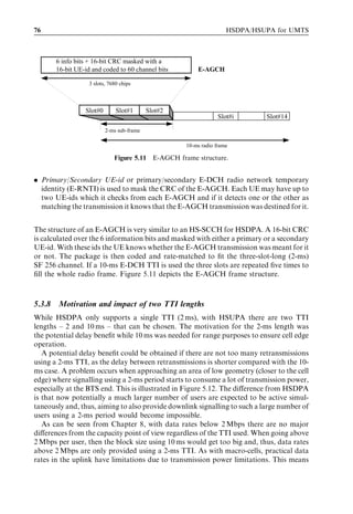
![HSUPA principles 77
Area where only a 10ms E-DCH/HSDPA serving cell
TTI is feasible
o l
ntr
co
H
DC PA
E- SD
H /H
DC CH
/D
D CH
E-
Area where both a 2ms and
a 10 ms TTI are feasible
Terminal
Figure 5.12 2-ms and 10-ms TTI applicability in a cell.
the 10-ms TTI is expected as the starting value for system deployment; this has also been
reflected in terminal capabilities (where a 2-ms TTI is optional for most categories).
5.4 Physical layer procedures
The physical layer operation procedure of HSUPA has fewer elements specified in the
physical layer specifications compared with HSDPA. One of the key reasons is that more
of the functionality regarding terminal transmission control is located in the MAC
specifications [9]. Physical layer procedures cover the handling of physical layer signal-
ling from the Node B and HSUPA operation in compressed mode. Further, the HARQ
operation procedure is covered in different parts of the specification in different channel
descriptions as well as different timing sections.
5.4.1 HARQ
The fundamental principle underlying HSUPA HARQ operation has a lot of similarities
to HSDPA in terms of retransmission combining. Now, as the link direction is different,
the soft buffer is maintained by the Node B instead of the terminal. The terminal will keep
unacknowledged data in memory, and the MAC layers trigger retransmission if the
physical layer provides a NACK as received from the Node Bs in the E-DCH active set.
Both soft (Chase) combining and incremental redundancy are available with HSUPA as
well (using the principles behind the combining methods covered in Chapter 4). The
fundamental difference in operation procedure is the synchronous nature of the HSUPA
HARQ process. As a function of the TTI being used – 2 ms or 10 ms – all the remaining
timing events are defined, including the number of HARQ processes. With a 10-ms TTI,
there are four HARQ processes, and the processing times are fixed within a 2-ms window.
The window results from the timing rule set for downlink signalling channel association
with uplink data transmissions. Depending on the uplink timing, downlink signalling
channels are set with the 2-ms resolution for the possible starting point. HARQ process](https://image.slidesharecdn.com/wileyhsdpahsupaforumts-12712250730845-phpapp02/85/Hsdpa-Hsupa-For-Umts-94-320.jpg)
![78 HSDPA/HSUPA for UMTS
E-HICH
14–16 ms 5.5–7.5 ms
DL
8 ms
ACK/NACK
E-DPCCH E-DPCCH
E-DCH E-DCH
UL
10 ms 30 ms (3 TTIs)
First retransmission
Figure 5.13 HSUPA HARQ process timing with a 10-ms TTI.
timing with a 10-ms TTI is shown in Figure 5.13, where the resulting four HARQ
processes are described.
There is no need to configure the number of HARQ processes, which gives clear
implementation guidance to Node B implementation in terms of which processing time
needs to be met in all cases. The Node B processing time requirement is thus approxi-
mately 14 ms, using the exact definition given in [2] and in [5]. The range up to 16 ms
cannot be easily utilized as the resulting time available depends on terminal uplink
timing, which is difficult to control in a network with mobility included. The extra
delay for a single retransmission is 40 ms (including the waiting/processing/signalling
time þ the additional TTI for retransmission). With a 2-ms TTI there are respectively
eight HARQ processes in use (as shown in Figure 5.14).
The use of a synchronous HARQ process removes the need to know as part of the data
stream which HARQ process is being used – as is the case for HSDPA to enable downlink
scheduling flexibility. With HSUPA the timing tells exactly which HARQ process is in
question, and the only indication needed is whether the data are new or a retransmission.
This is needed to avoid buffer corruption – either due to a signalling error (terminal
missing the ACK) or, especially in the case of soft handover, due to a Node B not being
aware of the possible ACK sent by another Node B in the active set.
E-HICH 3.5–5.5 ms
6.1–8.1 ms
DL
2 ms
ACK/NACK
E-DPCCH E-DPCCH
…
E-DCH E-DCH
UL
…
2 ms 14 ms (7 TTIs) First retransmission
Figure 5.14 HSUPA HARQ process timing with a 2-ms TTI.](https://image.slidesharecdn.com/wileyhsdpahsupaforumts-12712250730845-phpapp02/85/Hsdpa-Hsupa-For-Umts-95-320.jpg)
![HSUPA principles 79
HARQ control and
Packet soft combining
reordering AC
K/
NA
E-D CK
CH
d at
a
E-DCH data
ACK/NACK
RNC Correctly Node B Terminal
received packet
Figure 5.15 HSUPA ARQ operation in soft handover.
5.4.2 HARQ and soft handover
Operation with an active set larger than 1 causes additional implications for HARQ
operation. While with HSDPA only one Node B was involved in HARQ handling, with
HSUPA all the Node Bs in the active set are involved. HARQ operation is done using
similar rules to those for uplink power control. If the single Node B part of the active set
sends an ACK, then the information given to the MAC layer is that an ACK has been
received and the MAC layer will consider the transmission successful and move on to the
next packet. The principle underlying HARQ operation in soft handover is shown in
Figure 5.15. As the different Node Bs handle the process independently, packet ordering
cannot be preserved by them and, thus, has to be adjusted in the RNC. This is also
reflected in the protocol architecture – in the form of an additional MAC entity in the
RNC.
For NACKs from the non-serving cells mapping is defined as a zero-sequence and,
thus, NACKs are not really transmitted from cells other than serving cells. If the serving
cell is in softer handover with other cells defined as belonging to the same E-DCH radio
link set, then NACKs are transmitted from all of these cells in order to enable combining
in the receiver similar to that of the power control commands received in the softer
handover case. ACK/NACK mapping is described in detail in Section 5.3.5.
5.4.3 Measurements with HSUPA
While HSDPA does not directly introduce new terminal physical layer measurements
that need to be reported to the network, unless you count channel quality information
(CQI) as one, with HSUPA a new physical layer measurement is added that relates to
terminal power headroom. UE transmission power headroom (UPH) is defined in [6] as
being the ratio of the maximum UE transmission power and the corresponding DPCCH
code power. The maximum power is either according to the power level of the terminal
power class or a lower level if the maximum power is restricted by the UMTS Terrestrial
Radio Access Network (UTRAN). UPH reporting is illustrated in Figure 5.16.
UPH indicates the available power resources – that is, whether or not and by how
much the terminal could increase the data rate from the current situation. If the reported](https://image.slidesharecdn.com/wileyhsdpahsupaforumts-12712250730845-phpapp02/85/Hsdpa-Hsupa-For-Umts-96-320.jpg)
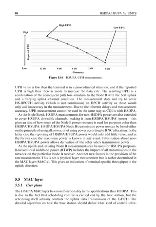
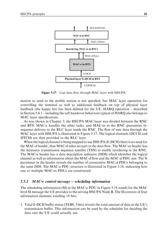
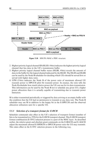
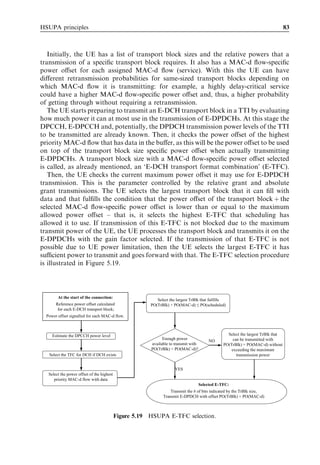
![84 HSDPA/HSUPA for UMTS
5.5.4 E-DCH coexistence with DCH
As described earlier, transport block processing for the E-DCH and DCH is completely
different and is carried over the air interface by completely separate physical channels,
too. Apart from one very important fact – that is, the shared power amplifier of the UE –
simultaneous transmission of the E-DCH and DCH could be considered to be coming
from two different UEs. There is only so much power the UE is capable of transmitting
and if the DCH is using some of it there is less for the E-DCH.
The interaction between the DCH and the E-DCH in simultaneous transmission from
the same UE is simply so that TFC selection is first done for the DCH and the power used
by doing this is, of course, no longer available for the E-TFC selection process. This
means that the DCH has an absolute first take right to the UE power resource, or the
DCH has absolute priority over the E-DCH. The reason for this is that the E-DCH is
designed for uplink packet access and, thus, if there are any circuit-switched services they
must be mapped to the DCH. As circuit-switched services are not very tolerant of sudden
and frequent data rate changes it makes sense to let, say, a normal AMR voice call to take
the power it needs and send it with that on DCH and use whatever is left for packet data
transmission on the E-DCH. The power allocation of the TFC and E-TFC selection
processes of the UE is illustrated in Figure 5.20. The TFC and E-TFC selection processes
are defined in [9]. It should be noted though that the maximum DCH data rate allowed by
the specification is 64 kbps when configured parallel to the E-DCH.
All of this has one notable impact on radio bearer mapping. If a DCH is configured
parallel to an E-DCH for a single UE, then the signalling radio bearer must also be
mapped to the DCH. This is due to the fact that the signalling radio bearer is the most
important bearer, and it would not be acceptable to let the power required to transmit a
voice frame prevent the transmission of a signalling message – that is, the SRB may only
be mapped to the E-DCH if there are no DCHs configured for the UE.
E-TFC selection can use the UE TX power
power left after TFC
selection, limited by
available power and Max UE TX power
scheduled maximum
Power available Node B scheduler controls the
Power available for for maximum relative power
DCH+E-DCH transmission E-DPCCH/E-DPDCH E-TFC selection may use
DPCCH + DPDCH
TFC selection allocates all power
the power it needs to Estimated DPCCH
transmit the DPDCH at a TX power
selected data rate
Figure 5.20 E-DCH and DCH power resource sharing.](https://image.slidesharecdn.com/wileyhsdpahsupaforumts-12712250730845-phpapp02/85/Hsdpa-Hsupa-For-Umts-101-320.jpg)
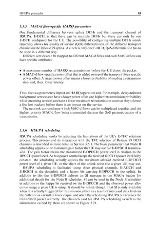
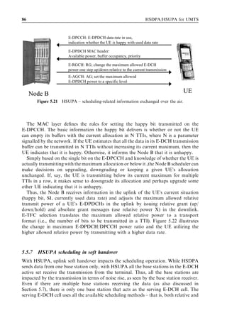
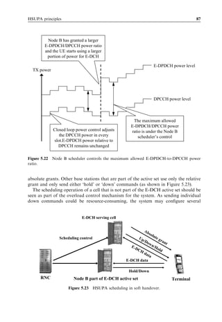
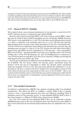
![HSUPA principles 89
5.6 Iub parameters
Similar to HSDPA operation, HSUPA also needs a large number of parameters to be
aligned between the terminal and the Node B. These are provided (as shown in Figure
5.24) to the Node B from the RNC, based on vendor-specific algorithms in the RNC and
on the terminal’s capability. These parameters can be broken down into the following
categories:
. Parameters for Node B resource allocation, to indicate, say, which codes are available
for the E-HICH/E-AGCH/E-RGCH.
. Scheduler parameters, to control scheduler behaviour, such as scheduling priority
indicator, maximum data rate, maximum RTWP value, or guaranteed bit rate.
. Terminal-specific parameters, such as the terminal’s capability, maximum bit rate,
puncturing limit, which code word on the HICH/E-AGCH/E-RGCH terminal is
listening to, or the TTI to be used. A 10-ms TTI could be used for all terminals,
but with a 2-ms TTI there will be a need to check the terminal’s capability and return
the reconfiguration to a 10-ms TTI when closer to the cell edge.
Respectively, terminal-specific parameters are then communicated by the RRC signal-
ling the terminal to have them aligned between the terminal and the Node B [9, 10]. From
the core network point of view, nothing else has changed from Release 99, except that
higher data rates are also enabled in the uplink direction compared with the theoretical 2-
Mbps or the practical 384-kbps uplink being used by HSDPA terminals.
There are a few parameters which are sent from the Node B towards the RNC that
relate to Node B HSUPA capability. The Node B can respond to an audit message,
say, from the RNC about HSUPA resource availability status. This is useful if Node B
resources depend on the other features being used or to see when the Node B might be
overloaded from the HSUPA resource point of view.
For the DCH case, there are some key differences with Iub interface usage. First of all,
only the so-called ‘silent mode’ is used – that is, the Node B will send a received data
packet to the RNC only after successfully decoding the packet. Empty frames indicating
failed decoding or a zero data rate will not be transmitted as is done with the DCH, with
the exception of the serving E-DCH cell when the maximum number of HARQ retrans-
missions is exceeded. The E-DCH serving cell will indicate a failed HARQ process when
UE capability,
scheduling
priority, resources, QoS
data rates … parameters
Control
PS
core
Iub Iu-ps
Data
Terminal Node B RNC
Figure 5.24 HSUPA parameters over the Iub interface.](https://image.slidesharecdn.com/wileyhsdpahsupaforumts-12712250730845-phpapp02/85/Hsdpa-Hsupa-For-Umts-106-320.jpg)
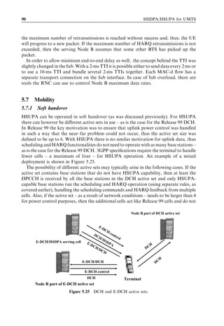
![HSUPA principles 91
take part in HARQ and scheduling operation. This allows the total number of additional
signalling channels the terminal has to listen to in soft handover to be limited. Obviously,
all the cells in the E-DCH active set must be in the DCH active set as well, but the DCH
active set may also contain cells that do not belong to the E-DCH active set if this is seen
useful by the network.
The change in serving E-DCH cell can be based on the same criteria as the change in
serving HSDPA cell. For this the measurement event – 1D – has already been modified in
Release 5 to allow reporting when the best serving cell changes. There is no obvious
reason why the serving E-DCH cell would not be the same as the serving HSDPA cell,
and this is also required to be the case in the specifications. The network may configure
the UE uplink/downlink operation so that HSDPA would not be used in the downlink
even if HSUPA is being used in the uplink. From the terminal capability point of view all
HSUPA-capable devices are required to support HSDPA as well [8]. A new measurement
event 1J can be used for active set management.
5.7.2 Compressed mode
Compressed mode handling using HSUPA depends on the TTI length. With a 2-ms TTI
the solution is simple, as the uplink E-DPDCH is not transmitted at all if compressed
mode overlaps partly or fully with the TTI, the solution being the same as with HSDPA.
Sub-channel timing is maintained and the retransmission is then postponed to the next
available TTI of the same HARQ sub-channel, preventing any sliding of HARQ process
timing. With a 10-ms TTI the solution has to be different, as otherwise a frequent
compressed mode patter could have suspended the data flow too critically, even fully
on some HARQ processes. In the 10-ms TTI case, terminal behaviour depends on such
cases as follows:
. If the initial transmission experiences a compressed mode transmit gap (TX GAP), the
retransmission will transmit the same number of slots in the TTI as shown in case A in
Figure 5.26. Only the same number of slots as the initial transmission will be utilized
and the terminal will use discontinuous transmission (DTX) for the E-DPDCH for the
extra slots (during which control channels are still transmitted).
0 1 2Slot 2Slot 2 TX GAP 11 121314
Slot 2 3 4 5 6 Slot 2 30 ms 0 1 2Slot 2Slot 2 7 8 9
Slot 2 3 4 5 6 DTX
A First retransmission
10 ms first transmission
Case B) Only retransmission is compressed
0 1 2Slot 2Slot 2 7 8 9 1011 12 1314
Slot 2 3 4 5 6 Slot 2Slot 2Slot 2 30 ms 0 1 2Slot 2Slot 2 7 8 TX GAP 1314
Slot 2 3 4 5 6
First retransmission
10 ms first transmission
B
Figure 5.26 HSUPA operation with compressed mode: in case A only the first TX is
compressed; in case B just the retransmission is compressed.](https://image.slidesharecdn.com/wileyhsdpahsupaforumts-12712250730845-phpapp02/85/Hsdpa-Hsupa-For-Umts-108-320.jpg)
![92 HSDPA/HSUPA for UMTS
. If a TX GAP occurs for the retransmission, then – as shown in case B in Figure 5.26 –
only as many slots as available will be used. The rate matching functionality will
assume for spreading factor selection and rate matching the same number of slots as
in the initial transmission, but will only transmit as many slots as actually available in
the frame [3].
The operation is simplified with the definition that the retransmission will always assume
the same number of slots for rate matching and spreading factor selection. From a
practical operation point of view, sending slots with reasonable energy per bit is also
preferable to sending at very high data rates (which would be subject to terminal
capabilities as well) for just a few slots. With downlink HSUPA signalling channels
(E-RGCH/E-AGCH/E-HICH), despite the terminal trying to grab most of the energy it
is allowed to ignore those slots that overlap with a downlink TX GAP.
Similarly to HSDPA, the use of compressed mode on E-DPDCH can be avoided.
There is a possibility to reconfigure to the DCH when performing inter-system or inter-
frequency measurements. From the network point of view, configuring from a 10-ms to a
2-ms TTI – to avoid dealing with compressed mode – is not typically a sensible thing to do
as inter-system and inter-frequency measurements are often needed at the point when the
terminal is closer to the coverage limit and, thus, is having its transmission power limited.
As discussed in Section 5.3.8, the link budget with signalling using a 2-ms TTI is worse
and, thus, does not suggest using 2 ms for typical cases of compressed mode.
5.8 UE capabilities and data rates
The same approach was chosen for HSUPA terminal capabilities as with HSDPA. The
terminal informs the network of one from six possible terminal categories instead of
signalling individual capabilities. The key differences between different categories are
related to the terminal’s multicode capability and to the support of a 2-ms TTI. All
terminal categories support the 10-ms TTI. The categories are shown in Table 5.8.
Table 5.8 HSUPA terminal categories.
Category Maximum number Supported TTIs Maximum data rate Maximum data rate
of E-DPDCHs and with a 10-ms TTI 1 with a 2-ms TTI 2
smallest spreading
factor
1 1 Â SF4 10 ms 0.72 Mbps N/A
2 2 Â SF4 2 and 10 ms 1.45 Mbps 1.45 Mbps
3 2 Â SF4 10 ms 1.45 Mbps N/A
4 2 Â SF2 2 and 10 ms 2 Mbps 2.91 Mbps
5 2 Â SF2 10 ms 2 Mbps N/A
6 2 Â SF2 þ 2 Â SF4 2 and 10 ms 2 Mbps 5.76 Mbps
1
Physical layer data rates.](https://image.slidesharecdn.com/wileyhsdpahsupaforumts-12712250730845-phpapp02/85/Hsdpa-Hsupa-For-Umts-109-320.jpg)
![HSUPA principles 93
Table 5.9 RLC layer data rates with 320-bit PDU size.
Category Maximum data rate with a 10-ms TTI 1 Maximum data rate with a 2-ms TTI 1
1 0.672 Mbps N/A
2 1.376 Mbps 1.280 Mbps
3 1.376 Mbps N/A
4 1.888 Mbps 2.720 Mbps
5 1.888 Mbps N/A
6 1.888 Mbps 5.440 Mbps
1
Data rates offered by the RLC layer assuming 320-bit PDU size and typical MAC header.
As shown in Table 5.9, all categories except category 1 can carry out multicode
transmission. With category 6 the notation in Table 5.8 means that two E-DPDCHs
are transmitted with a spreading factor of 4 and two with a spreading factor of 2.
Additionally, [7] defines the minimum total terminal RLC/MAC buffer size for combined
HSDPA and HSUPA operation. The values range from 50 kbytes (HSPDA category 12
and HSUPA category 1) to 400 kbytes (HSDPA category 10 and HSUPA category 6).
The maximum uplink DCH capability when configured simultaneously with HSUPA
is 64 kbps for all the UE categories.
There is a similar impact on bit rates above the physical layer due to the overhead on
the MAC and RLC layers, as is the case with HSDPA. Thus, data rates above the RLC
layer are reduced compared with maximum physical layer data rates. The resulting RLC
layers for different categories are shown in Table 5.9. In a few cases, a 2-ms TTI suffers a
bit more as individual TTI has smaller payload and relative overhead is slightly higher.
5.9 References and list of related 3GPP specifications
[1] H. Holma and A. Toskala (eds) (2004), WCDMA for UMTS (3rd edn), John Wiley &
Sons.
[2] 3GPP, Technical Specification Group RAN, Physical channels and mapping of transport
channels onto physical channels (FDD), 3GPP TS 25.211 version 6.7.0, Release 6, available
at www.3gpp.org
[3] 3GPP, Technical Specification Group RAN, Multiplexing and channel coding (FDD),
3GPP TS 25.212 version 6.7.0, Release 6, available at www.3gpp.org
[4] 3GPP, Technical Specification Group RAN, Spreading and modulation (FDD), 3GPP TS
25.213 version 6.4.0, Release 6, available at www.3gpp.org
[5] 3GPP, Technical Specification Group RAN, Physical layer procedures (FDD), 3GPP TS
25.214 version 6.7.1, Release 6, available at www.3gpp.org
[6] 3GPP, Technical Specification Group RAN, Physical layer – measurements (FDD), 3GPP
TS 25.215 version 6.4.0, Release 6, available at www.3gpp.org
[7] 3GPP, Technical Specification Group RAN, UE radio access capabilities definition, 3GPP
TS 25.306 version 6.7.0, Release 6, available at www.3gpp.org
[8] 3GPP, Technical Specification Group RAN, FDD enhanced uplink; Overall description;
Stage 2, 3GPP TS 25.309 version 6.4.0, Release 6, available at www.3gpp.org](https://image.slidesharecdn.com/wileyhsdpahsupaforumts-12712250730845-phpapp02/85/Hsdpa-Hsupa-For-Umts-110-320.jpg)
![94 HSDPA/HSUPA for UMTS
[9] 3GPP, Technical Specification Group RAN, Medium Access Control (MAC) protocol
specification, 3GPP TS 25.321 version 6.7.0, Release 6, available at www.3gpp.org
[10] 3GPP, Technical Specification Group RAN, Radio Resource Control (RRC) protocol
specification, 3GPP TS 25.331 version 6.8.0, Release 6, available at www.3gpp.org
[11] 3GPP, Technical Specification Group RAN, Iub, 3GPP TS 25.433 version 6.8.0, Release 6,
available at www.3gpp.org](https://image.slidesharecdn.com/wileyhsdpahsupaforumts-12712250730845-phpapp02/85/Hsdpa-Hsupa-For-Umts-111-320.jpg)
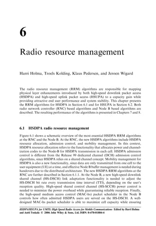
![96 HSDPA/HSUPA for UMTS
RNC Node-B
Resource HS-DSCH link
allocation adaptation
Admission Iub Packet
control scheduling
Mobility HS-SCCH
management power control
Figure 6.1 Overview of the most relevant HSDPA RRM algorithms.
an attractive end user experience. The new HSDPA RRM algorithms at the Node B are
discussed in Section 6.1.2. Note that the Third Generation Partnership Project (3GPP)
only defines the interfaces and minimum UE performance requirements. Hence, network
equipment manufacturers can individually design their Node B and RNC RRM algo-
rithms according to market demands.
6.1.1 RNC algorithms
6.1.1.1 Resource allocation
Before the Node B can start transmitting data on the HS-DSCH, the controlling RNC
needs to allocate channelization codes and power for the transmission of HSDPA. As a
minimum, one HS-SCCH code with a spreading factor (SF) of 128 and one HS-PDSCH
code with SF16 should be allocated to the Node B. The RNC and Node B signal to one
another using the Node B Application Part (NBAP) protocol specified by 3GPP in [1].
The resources are allocated by sending an ‘NBAP: Physical shared channel reconfigura-
tion request’ message from the controlling RNC to the Node B (as shown in Figure 6.2).
Hence, the allocation of channelization codes for HSDPA transmission only requires
signalling between the RNC and the Node B. In general, it is advantageous to allocate as
many high-speed physical downlink shared channel (HS-PDSCH) codes to the Node B
as possible, since the spectral efficiency of the HS-DSCH is thereby improved. On the
other hand, channelization codes reserved for HS-PDSCH transmission cannot be
simultaneously used for transmission of Release 99 channels, so allocation of many
HS-PDSCH codes might eventually result in call blocking of Release 99 users. For-
tunately, if channelization code congestion is detected, the controlling RNC can quickly
Controlling NBAP: Physical shared channel
Node B
RNC reconfiguration request
Figure 6.2 Signalling for HSDPA resource allocation.](https://image.slidesharecdn.com/wileyhsdpahsupaforumts-12712250730845-phpapp02/85/Hsdpa-Hsupa-For-Umts-113-320.jpg)
![Radio resource management 97
Carrier transmission power
Maximum power
Total carrier
power HSDPA
PtxTarget
Non-real time R99
Non-HSDPA
power
Real time R99
Common channels
Figure 6.3 Illustration of downlink power budget.
release some of the allocated HS-PDSCH codes to prevent blocking of Release 99 voice
or video connections.
HS-DSCH transmission to multiple users in parallel during a single TTI requires
multiple HS-SCCH codes and multiple HS-PDSCH codes. Code multiplexing is typically
found useful for scenarios where a Node B has more HS-PDSCH codes allocated than
what is supported by HSDPA mobiles; the Node B may support 10–15 HS-PDSCH
codes while the HSDPA terminal supports only 5 HS-PDSCH codes. The algorithm for
allocation of HS-SCCH codes to the Node B can therefore be derived as a function of
allocated HS-PDSCH codes and HSDPA UE categories in the cell. The performance
results are presented in Chapter 7 as a function of the number of channelization codes
reserved for HSDPA.
In most cases, the most scarce downlink transmission resource is power. Figure 6.3
shows the downlink power budget for a cell with transmission on both HSDPA and
Release 99 channels. The power budget consists of the power needed for common
channels such as the P-CPICH, power for Release 99 DCH transmissions, and power
for HSDPA transmission. As discussed in [2], the power for real time DCHs is managed
by RNC admission control, while non-real time DCHs are controlled by the RNC packet
scheduler. The power for non-real time DCH is characterized as controllable power since
it can be adjusted via bit rate modifications, while the power for common channels and
real time DCH is considered to be non-controllable. An example power allocation case is
illustrated in Figure 6.3. Assuming a power-based RRM paradigm, the RNC RRM
algorithm aims at keeping the total power for all Release 99 channels below PtxTarget
[2]. In order to allow implementation of such schemes with HSDPA as well, the Node B
can be configured to report average measurements of non-HSDPA power per carrier (as
illustrated in Figure 6.3). Based on these measurements, the RNC is able to conduct
admission control and packet scheduling for Release 99 channels in cells with simul-
taneous HSDPA transmission (see, e.g., the studies in [6] and [8]).](https://image.slidesharecdn.com/wileyhsdpahsupaforumts-12712250730845-phpapp02/85/Hsdpa-Hsupa-For-Umts-114-320.jpg)
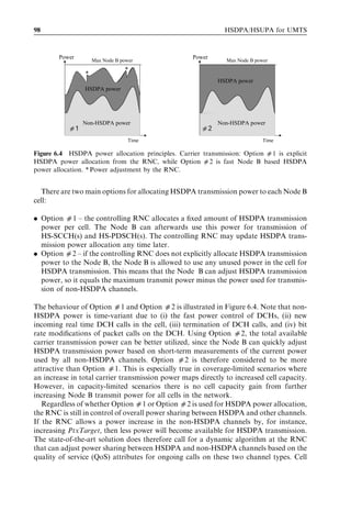
![Radio resource management 99
capacity performance results for HSDPA and the DCH are presented in Chapter 7 for
different power allocations between those two channel types.
6.1.1.2 QoS parametrization
QoS for Release 99 DCHs is conducted as a function of the user’s traffic class (TC), traffic
handling priority (THP), allocation retention priority (ARP), and potentially also other
Universal Mobile Telecommunications System (UMTS) bearer attributes (as discussed
in [2], [3]). These QoS parameters from the Iu interface are not available in the Node B for
MAC-hs packet scheduling. New QoS parameters have been defined for the Iub interface
between the RNC and the Node B. HSDPA QoS parameters in the Iub are:
. guaranteed bit rate (GBR);
. scheduling priority indicator (SPI); and
. discard timer (DT).
Figure 6.5 illustrates 3GPP QoS parameters and their interfaces. 3GPP neither defines
how parameter mapping is designed in the RNC, nor how the QoS parameters are used
by the MAC-hs packet scheduler.
Scheduling priority indicator (SPI) takes values in the range [0; 1; . . . ; 15], where a high
number indicates high priority and vice versa. The DT specifies the maximum time that a
packet is allowed to be buffered in the Node B’s MAC-hs before it should be discarded.
For the conversational and streaming traffic class, the HSDPA GBR parameter can be
set according to the bit rate requirement specified in the UMTS bearer attribute for this
traffic class. A high SPI could be allocated to video streaming or other real time services,
while general Internet access applications could be assigned a low SPI value. 3GPP
specifications also allow implementation of advanced options where the SPI is adjusted
dynamically during a packet call. As will be discussed next, the value of the GBR and SPI
for new HSDPA users who are requesting access can also be used in the HSDPA
admission control decision.
6.1.1.3 Admission control
HSDPA admission control is the functionality that determines whether new users with
HSDPA terminals can be granted access to the cell and whether they will be served
using HSDPA or the DCH. The admission control decision is taken by the RNC. In case
• Traffic class TC Scheduling priority indicator SPI Node B
SGSN RNC •
• Traffic handling priority THP • Guaranteed bit rate GBR
• Allocation and retention priority ARP • Discard timer DT
• Guaranteed bit rate GBRIu
Iu-PS Iub
Figure 6.5 3GPP QoS parameters in the Iu-PS and Iub interfaces.](https://image.slidesharecdn.com/wileyhsdpahsupaforumts-12712250730845-phpapp02/85/Hsdpa-Hsupa-For-Umts-116-320.jpg)
![100 HSDPA/HSUPA for UMTS
Admission
control in RNC Node B UE
Total carrier power
Non-HSDPA power
HS-DSCH required power
Pilot power measurements
Figure 6.6 Sketch of measurements and parameters applicable for HSPDA admission control [5].
of circuit-switched services, like AMR speech or video, it is obvious to stick with the
DCH. For packet-switched services the algorithm in the RNC needs to consider the
QoS parameters provided by the core network as well as the general resource situation
in the network. If only best effort traffic with no strict QoS requirements are transmitted
on HSDPA, then the admission control algorithm can be made fairly simple by only
checking the availability of RNC and Node B hardware resources to serve a new HSDPA
user. If more demanding services with stricter QoS requirements are considered for
HSDPA, then a more advanced admission control algorithm is needed to ensure that
the QoS requirements for existing HSDPA users in the cell as well as the requirements of
the new user can be fulfilled after the potential admission. Examples of quality-based
HSDPA access control algorithms are studied in [5]–[7], where the QoS attributes of new
HSDPA users are taken into account in admission control decisions. Hence, using this
type of algorithm, high-priority users tend to experience a lower blocking probability
than low-priority users.
Figure 6.6 shows an example of the measurements and parameters that are available
for HSDPA admission control in the RNC: the Node B reports the total average carrier
transmit power and the non-HSDPA transmit power. Given these two measurements,
the RNC can compute the amount of available HSDPA transmit power in the cell. The
Node B also reports the HS-DSCH power needed to serve all the existing HSDPA users
in the cell with their guaranteed bit rates. Finally, the new user requesting HSDPA access
sends a pilot common pilot channel (CPICH) Ec =N0 measurement report to the RNC.
The latter measurement can be used by the RNC to estimate the HS-DSCH signal quality
of the user. Given these measurements – together with the user’s QoS attributes – the
RNC can estimate whether there is HSDPA capacity available to grant the new user
access without violating the QoS requirements for the existing users in the cell [5]. As
discussed in [4]–[5], such an HSDPA admission control algorithm efficiently supports
high-quality streaming and VoIP services on HSDPA. Finally, note that the non-
HSDPA power measurement from the Node B can also be used for conventional
power-based admission control of the Release 99 channels that coexists on the same
carrier [8].
6.1.1.4 Mobility management
HSDPA does not use soft handover, since HS-DSCH and HS-SCCH transmission take
place only from a single cell, called the ‘serving HS-DSCH cell’. The RNC determines the](https://image.slidesharecdn.com/wileyhsdpahsupaforumts-12712250730845-phpapp02/85/Hsdpa-Hsupa-For-Umts-117-320.jpg)
![Radio resource management 101
serving HS-DSCH cell for the active HSDPA UE. The serving HS-DSCH cell is one of
the cells in the UE’s active set. A synchronized change in the serving HS-DSCH cell is
supported between the UTRAN and the UE. This feature allows benefitting from the
HSDPA service with full coverage and with full mobility [7]. The serving HS-DSCH cell
may be changed without updating the user’s active set for Release 99 dedicated channels
or in combination with establishment, release, or reconfiguration of the DCHs. An
HS-DSCH serving cell change is typically based on measurement reports from the
UE. 3GPP Release 5 includes a new measurement procedure to inform the RNC of
the best serving HS-DSCH cell.
In the following subsections, we briefly discuss the new UE measurement event for
supporting mobility for HSDPA users, as well as outline the procedures for intra and
inter Node B HS-DSCH to HS-DSCH handover. Finally, we address handover from
HS-DSCH to the Release 99 DCH. Inter-frequency handovers with compressed mode
measurements are also supported for HSDPA users but are not considered in this
section [2].
6.1.1.4.1 Measurement event for best serving HS-DSCH cell
The serving RNC determines what cells are in the active set for transmission of DCHs.
The serving RNC makes the handover decisions directly based on the CPICH meas-
urement reports from the UE. A measurement event ‘1d’ has been defined for HSDPA –
that is, a change in best serving HS-DSCH cell [9]. This measurement reports the
CPICH Ec =N0 of the best cell, and is triggered when the best cell changes (as illustrated
in Figure 6.7). It is possible to configure this measurement event so that all cells in the
user’s candidate set are taken into account, or to restrict the measurement event so that
only the current cells in the user’s active set for DCHs are considered. Usage of a
hysteresis margin to avoid fast change in the serving HS-DSCH cell is also possible
for this measurement event, as well as specification of a cell-individual offset to favour
certain cells – for instance, to extend their HSDPA coverage area.
CPICH Ec/I0 ∆T = time to trigger
∆D = handover delay
H = hysteresis
Ec/I0 of cell 1
Ec/I0 of cell 2
H
∆T ∆D
Time
HS-DSCH from cell 1 HS-DSCH from cell 2
Figure 6.7 Graphical illustration of best serving HS-DSCH cell measurement from the user.](https://image.slidesharecdn.com/wileyhsdpahsupaforumts-12712250730845-phpapp02/85/Hsdpa-Hsupa-For-Umts-118-320.jpg)
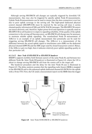
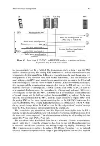
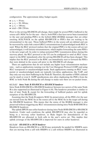
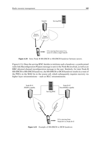
![106 HSDPA/HSUPA for UMTS
Table 6.1 Summary of HSDPA handover types and their characteristics.
Intra Node B Inter Node B HS-DSCH to DCH
HS-DSCH to HS-DSCH HS-DSCH to HS-DSCH
Handover
Typically by UE, but possibly also by Node-B
measurement
Handover
By serving RNC
decision
Packet Packets forwarded Packets not forwarded. RLC retransmissions
retransmissions from source MAC-hs to RLC retransmissions used from SRNC
target MAC-hs used from SRNC
Packet losses No No, when RLC No, when RLC
acknowledged mode is acknowledged mode
used, or when duplicate is used
packets are sent on
RLC unacknowledged
mode
Uplink HS-DPCCH can use HS-DPCCH received by
HS-DPCCH softer handover one cell
Release 5 specifications also support implementation of handover from the DCH to
the HS-DSCH. This handover type may, for instance, be used if a user is moving from a
non-HSDPA capable cell to an HSDPA-capable cell.
6.1.1.4.5 Summary of intra-frequency HSDPA handover characteristics
Table 6.1 presents a summary of the different handover modes and their characteristics.
Various performance results for HSDPA over the Release 99 DCH are presented in [7]
for users with different active set sizes, and for different HSDPA handover strategies.
6.1.2 Node B algorithms
6.1.2.1 HS-DSCH link adaptation techniques
The HS-DSCH link adaptation algorithm at the Node B adjusts the transmit bit rate
on the HS-DSCH every TTI when a user is scheduled for transmission. Ideally, the
HS-DSCH transmit bit rate should be adjusted as a function of the per-TTI HS-DSCH
signal-to-interference plus noise ratio (SINR) experienced at the user end. The general
principle underlying HS-DSCH link adaptation is illustrated in Figure 6.12.
Various sources contribute to variance of HS-DSCH SINR even though the
HS-DSCH transmit power is assumed to be constant. The different factors are illustrated
in Figure 6.13. The total transmit power from the serving HS-DSCH cell is time-variant
due to the transmission of power-controlled DCHs, the downlink radio channel is time-
variant if the user is moving, and, finally, the other-cell interference experienced at the](https://image.slidesharecdn.com/wileyhsdpahsupaforumts-12712250730845-phpapp02/85/Hsdpa-Hsupa-For-Umts-123-320.jpg)
![Radio resource management 107
Channel quality information (CQI)
transmitted on HS-DPCCH
HS-DSCH link
adaptation
Fading channel
2
1 Time
Figure 6.12 HS-DSCH link adaptation principle: 1 ¼ the UE reports low-quality channel
information and the Node B allocates a low bit rate; 2 ¼ the UE reports high-quality channel
information and the Node B allocates a high bit rate.
Time-varying Time-varying
total transmit other-cell
power interference
Serving HS- Time-varying
DSCH cell radio channel Σ HSDPA user
Thermal noise
HS-DPCCH
signalling delay
and errors
Figure 6.13 Block diagram showing the received signal at the HSDPA user end and reporting of
the CQI to the serving HS-DSCH cell.
user end is also time-variant. For the purpose of HS-DSCH link adaptation, the UE
periodically sends a CQI to the serving HS-DSCH cell on the uplink HS-DPCCH (as
described in Chapter 4). The CQI indicates the maximum transport block size that can be
received correctly with at least 90% probability. This information is signalled via a CQI
index in the range from 0 to 31, where each step corresponds appoximately to a 1-dB step
in HS-DSCH SINR [10].](https://image.slidesharecdn.com/wileyhsdpahsupaforumts-12712250730845-phpapp02/85/Hsdpa-Hsupa-For-Umts-124-320.jpg)
![108 HSDPA/HSUPA for UMTS
RNC Node B UE
NBAP message: P-CPICH power + Γ
BLER target
Outer loop HS- Inner loop HS- HS-DSCH
DSCH link DSCH link HSDPA user
adaptation adaptation
ACK/NACK/DTX CQI HS-DPCCH
RRC message: Γ
Figure 6.14 Block diagram for the HS-DSCH link adaptation algorithm at the Node B.
A simple link adaptation algorithm would directly follow the CQI values reported by
the UE. However, there may be a need to adjust the UE-reported CQI by adding an offset
for the following reasons. The HS-DSCH transmit power from the Node B to the user
might be different from the assumed HS-DSCH transmit power by the UE at the time
it derived the CQI report. The UE assumes that HSDPA power equals the power of the
primary common pilot channel (P-CPICH) plus G, where G is a power offset parameter
signalled to the UE via RRC signalling from the RNC.
The effect of feedback delays on link adaptation performance has previously been
addressed in [11], [12]. The conclusion from those studies indicate a need for an outer
loop HS-DSCH link adaptation algorithm to further adjust the CQI index received from
a user before applying it for adjustment of the HS-DSCH transmission format.
The outer loop algorithm can be based on ACKs/NACKs from past transmissions.
The algorithm adjusts the offset values to ascertain the average targetted retransmission
probability. Too many retransmissions add an unnecessary delay while too few indicate
that the transport block sizes used are not large enough, unnecessarily lowering through-
put. Outer loop HS-DSCH link adaptation can be based on the same principle as
the Release 99 outer loop power control algorithms that were first published in [13].
Examples of outer loop HS-DSCH link adaptation algorithms are studied in [14], [15].
The HS-DSCH link adaptation algorithm is summarized in the simplified block diagram
in Figure 6.14.
6.1.2.2 HS-SCCH power control
Reliable reception quality of the HS-SCCH is important since the transport block on the
HS-DSCH can only be decoded if the HS-SCCH has first been correctly received.
Therefore, sufficient power should be allocated to transmission of the HS-SCCH to
ensure reliable reception. On the other hand, it is also desirable to reduce HS-SCCH
transmission power to lessen interference levels in the network. Hence, it is generally
recommended to have HS-SCCH power controlled every TTI, in which HS-SCCH
transmit power is adjusted such that the desired user has a high probability of correctly
decoding the channel (see Figure 6.15). A large amount of HS-SCCH power is used for](https://image.slidesharecdn.com/wileyhsdpahsupaforumts-12712250730845-phpapp02/85/Hsdpa-Hsupa-For-Umts-125-320.jpg)
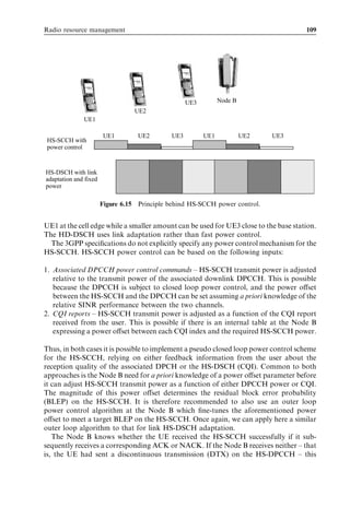
![110 HSDPA/HSUPA for UMTS
Node B UE
BLER target
Outer loop HS- Inner loop HS- HS-SCCH
SCCH power SCCH power HSDPA user
control control
ACK/NACK/DTX CQI HS-DPCCH
Figure 6.16 Block diagram for HS-SCCH power control algorithm.
implies that the UE did not detect the HS-SCCH transmission. This information can be
used for HS-SCCH power control. ACK/NACK reporting is further enhanced in 3GPP
Release 6 where the UE first sends a specific pre-amble message for an ACK/NACK to
help the Node B distinguish it from a DTX.
Figure 6.16 shows a simplified block diagram that summarizes the HS-SCCH
power control algorithm at the Node B. The HS-SCCH power control algorithm is
connection-specific. The design, performance, and power control of the HS-SCCH has
been further studied in [16], [17]. HS-SCCH performance results are furthermore pre-
sented in Chapter 7.
6.1.2.3 Packet scheduler
This section presents the functionality of the packet scheduler and introduces the
different types of scheduling algorithms and explains the trade-offs in terms of user
bit rate and cell capacity.
6.1.2.3.1 Basic theory
The basic problem a packet scheduler has is how to share the available resources to the
pool of users eligible to receive data. A commonly used formulation to describe this
challenge is the one proposed by Kelly [19]. Kelly uses the concept of a utility function,
Un ðrn Þ, where n denotes a particular HSDPA user and rn is the average throughput for
the nth user. Simply put, the utility function is a measure of the ‘happiness or satisfaction’
gained from being scheduled. The best scheduling solution is the one that maximizes the
sum of utility functions for all the users at any given time. The sum of the utility functions
is called the ‘objective function’.
Assuming that a proper utility function, Un ðrn Þ, has been defined, another challenge
lies in the time-variant behaviour of the cellular system. Each user’s channel capacity, as
well as the total cell capacity, varies over time. It was shown in [20] that the best that one
can do is to use a gradient search algorithm, which aims at further maximizing the
objective function for each scheduling decision. Hence, the system should schedule the
HSDPA user in the next TTI that fulfills [20]:
@Un ðrn Þ
n à ¼ arg maxn fMn g; where Mn ¼ dn Á ð6:1Þ
@rn](https://image.slidesharecdn.com/wileyhsdpahsupaforumts-12712250730845-phpapp02/85/Hsdpa-Hsupa-For-Umts-127-320.jpg)
![Radio resource management 111
Here, Mn denotes the so-called scheduling metric, dn is the instantaneous data rate that
HSDPA user number n can support in the next TTI. Note that dn is obtained by
consulting the HS-DSCH link adaptation algorithm (as discussed in Section 6.1.2.1).
The throughput delivered to HSDPA users in the past can be updated every TTI for all
users with a recursive expression (exponential smoothing); that is:
ð1 À aÞrn;old þ adn if user n is served
rn ¼
ð1 À aÞrn;old otherwise
where rn;old is the old value of rn and a is the forgetting factor. Hence, a À1 equals the
equivalent averaging period in a number of TTIs for the exponential smoothing filter.
Throughput calculation for a user is only done for periods of time when the user has data
in the Node B buffer. This is important for stability of QoS-aware packet scheduling
methods which would otherwise try to compensate for inactive users with no data to
transmit.
6.1.2.3.2 Packet scheduler algorithms
Different classical packet schedulers from the literature are listed in Table 6.2 according
to their utility and scheduling policy function. The round robin (RR) scheduler is a
Table 6.2 Packet scheduling principles.
Scheduler Utility function, Un ðrn Þ Scheduling metric, Mn
Round robin (RR) 1 0
Maximum C/I or rn dn
throughput (max-C/I)
dn
Proportional fair (PF) logðrn Þ
rn
[19], [21], [23], [24], [27]
Minimum bit rate rn þ ð1 À exp½À](https://image.slidesharecdn.com/wileyhsdpahsupaforumts-12712250730845-phpapp02/85/Hsdpa-Hsupa-For-Umts-128-320.jpg)
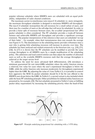
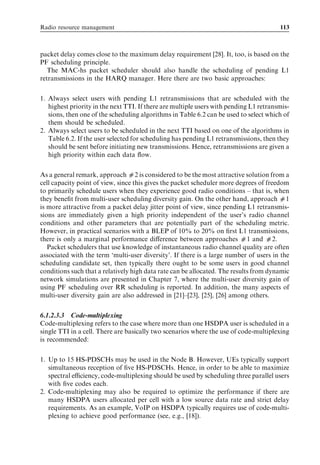
![ðrn À rmin ÞÞŠ
scheduling (min-GBR) [20]
1
Minimum bit rate logðrn Þ þ ð1 À exp½À](https://image.slidesharecdn.com/wileyhsdpahsupaforumts-12712250730845-phpapp02/85/Hsdpa-Hsupa-For-Umts-131-320.jpg)
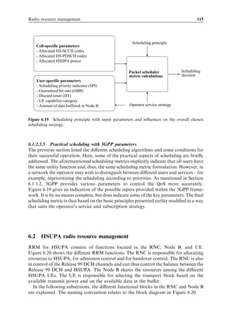
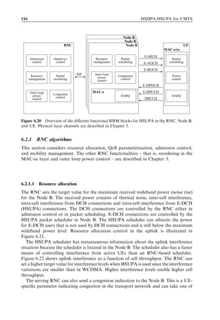
![ðrn À rmin ÞÞ
rn
scheduling with
proportional fairness
(min-GBR þ PF)
dHOL;n Àlogðn Þ Á dHOL;n
Maximum delay scheduling Àlogðn Þ logðrn Þ dn
dreq;n rn Á dreq;n
(max-Del) [28]
rmin ¼ Minimum bit rate target – for example, the guaranteed bit rate (GBR);](https://image.slidesharecdn.com/wileyhsdpahsupaforumts-12712250730845-phpapp02/85/Hsdpa-Hsupa-For-Umts-134-320.jpg)
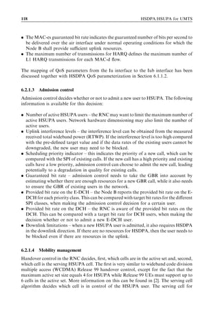
![¼ 0:5 [20]);
dHOL;n ¼ Head-of-line packet delay;
dreq;n ¼ Maximum packet delay requirement;
n ¼ Violation probability (or aggressive factor) for the algorithm [28].](https://image.slidesharecdn.com/wileyhsdpahsupaforumts-12712250730845-phpapp02/85/Hsdpa-Hsupa-For-Umts-136-320.jpg)
![112 HSDPA/HSUPA for UMTS
popular reference scheduler where HSDPA users are scheduled with an equal prob-
ability, independent of radio channel conditions.
The maximum carrier-to-interference ratio (max-C/I) scheduler or, more stringently,
the maximum throughput scheduler is designed to maximize HSDPA cell throughput.
The max-C/I scheduler monopolizes the cell resources for a small subset of users, and
there may be a number of users at the cell edge that will never be scheduled. In order to
provide a fairer split of resources between users, the so-called ‘proportional fair’ (PF)
packet scheduler is often considered. The PF scheduler provides a trade-off between
fairness and achievable HSDPA cell throughput and provides a significant coverage
extension. The popular interpretation of this relation is that users are scheduled ‘on top
of their fades’ – for example, when their instantaneous data rate exceeds the average
(see Figure 6.17). The denominator in the scheduling metric provides robustness since a
user who is getting little scheduling resources will increase its priority over time. The
scheduler has been analysed and studied extensively in the literature (see, e.g., [19], [21],
[24]). In [27] it is shown that the PF scheduler can be modified to provide the same
average throughput to all HSDPA users by a simple modification of the scheduling
policy. The admission and load control entities can then adjust the number of allocated
users as well as the available HSDPA resources such that the average throughput is
achieved at the target service level.
To address the need for more advanced QoS differentiation, [20] introduces a
minimum guaranteed bit rate (min-GBR) scheduler where the utility function returns
a relatively low value for cases where the user’s experienced throughput is below the
GBR, while the utility function only increases moderately for throughputs experienced
higher than the GBR. By adjusting the value of](https://image.slidesharecdn.com/wileyhsdpahsupaforumts-12712250730845-phpapp02/85/Hsdpa-Hsupa-For-Umts-137-320.jpg)
![(see Table 6.2), it is possible to control
how aggressive the MAC-hs packet scheduler should be if the bit rate offered to the
HSDPA user drops below the GBR. In Table 6.2, a second variant is also included which
adds the basic PF scheduling principle. Other possibilities for defined utility functions are
presented in, for example, [20]. The last scheduler presented in Table 6.2 aims at fulfilling
packet delay requirements by increasing the scheduling priority when the head-of-line
Scheduled user
TTIs [2 ms]
UE 1 fading
UE 2 fading
UE 1 UE 2 UE 1 UE 2
Figure 6.17 Principle underlying proportional fair scheduling with a 3-TTI delay.](https://image.slidesharecdn.com/wileyhsdpahsupaforumts-12712250730845-phpapp02/85/Hsdpa-Hsupa-For-Umts-138-320.jpg)
![Radio resource management 113
packet delay comes close to the maximum delay requirement [28]. It, too, is based on the
PF scheduling principle.
The MAC-hs packet scheduler should also handle the scheduling of pending L1
retransmissions in the HARQ manager. Here there are two basic approaches:
1. Always select users with pending L1 retransmissions that are scheduled with the
highest priority in the next TTI. If there are multiple users with pending L1 retransmis-
sions, then one of the scheduling algorithms in Table 6.2 can be used to select which of
them should be scheduled.
2. Always select users to be scheduled in the next TTI based on one of the algorithms in
Table 6.2. If the user selected for scheduling has pending L1 retransmissions, then they
should be sent before initiating new transmissions. Hence, retransmissions are given a
high priority within each data flow.
As a general remark, approach 02 is considered to be the most attractive solution from a
cell capacity point of view, since this gives the packet scheduler more degrees of freedom
to primarily schedule users when they experience good radio conditions – that is, when
they benefit from multi-user scheduling diversity gain. On the other hand, approach 01
is more attractive from a packet delay jitter point of view, since pending L1 retransmis-
sions are immediately given a high priority independent of the user’s radio channel
conditions and other parameters that are potentially part of the scheduling metric.
However, in practical scenarios with a BLEP of 10% to 20% on first L1 transmissions,
there is only a marginal performance difference between approaches 01 and 02.
Packet schedulers that use knowledge of instantaneous radio channel quality are often
associated with the term ‘multi-user diversity’. If there is a large number of users in the
scheduling candidate set, then typically there ought to be some users in good channel
conditions such that a relatively high data rate can be allocated. The results from dynamic
network simulations are presented in Chapter 7, where the multi-user diversity gain of
using PF scheduling over RR scheduling is reported. In addition, the many aspects of
multi-user diversity gain are also addressed in [21]–[23], [25], [26] among others.
6.1.2.3.3 Code-multiplexing
Code-multiplexing refers to the case where more than one HSDPA user is scheduled in a
single TTI in a cell. There are basically two scenarios where the use of code-multiplexing
is recommended:
1. Up to 15 HS-PDSCHs may be used in the Node B. However, UEs typically support
simultaneous reception of five HS-PDSCHs. Hence, in order to be able to maximize
spectral efficiency, code-multiplexing should be used by scheduling three parallel users
with five codes each.
2. Code-multiplexing may also be required to optimize the performance if there are
many HSDPA users allocated per cell with a low source data rate and strict delay
requirements. As an example, VoIP on HSDPA typically requires use of code-multi-
plexing to achieve good performance (see, e.g., [18]).](https://image.slidesharecdn.com/wileyhsdpahsupaforumts-12712250730845-phpapp02/85/Hsdpa-Hsupa-For-Umts-139-320.jpg)
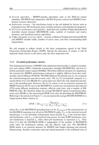
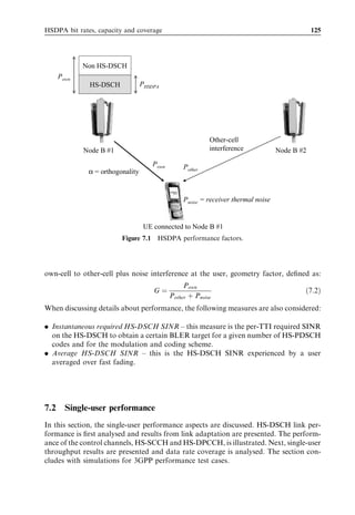
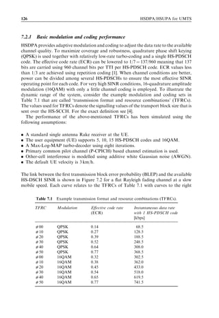
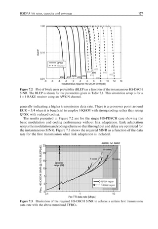
![118 HSDPA/HSUPA for UMTS
. The MAC-es guaranteed bit rate indicates the guaranteed number of bits per second to
be delivered over the air interface under normal operating conditions for which the
Node B shall provide sufficient uplink resources.
. The maximum number of transmissions for HARQ defines the maximum number of
L1 HARQ transmissions for each MAC-d flow.
The mapping of QoS parameters from the Iu interface to the Iub interface has been
discussed together with HSDPA QoS parameterization in Section 6.1.1.2.
6.2.1.3 Admission control
Admission control decides whether or not to admit a new user to HSUPA. The following
information is available for this decision:
. Number of active HSUPA users – the RNC may want to limit the maximum number of
active HSUPA users. Network hardware dimensioning may also limit the number of
active users.
. Uplink interference levels – the interference level can be obtained from the measured
received total wideband power (RTWP). If the interference level is too high compared
with the pre-defined target value and if the data rates of the existing users cannot be
downgraded, the new user may need to be blocked.
. Scheduling priority indicator – this indicates the priority of a new call, which can be
compared with the SPI of existing calls. If the new call has a high priority and existing
calls have a low priority, admission control can choose to admit the new call, leading
potentially to a degradation in quality for existing calls.
. Guaranteed bit rate – admission control needs to take the GBR into account by
estimating whether there are enough resources for a new GBR call, while it also needs
to ensure the GBR of existing users in the network.
. Provided bit rate on the E-DCH – the Node B reports the provided bit rate on the E-
DCH for each priority class. This can be compared with target bit rates for the different
SPI classes, when making the admission control decision for a certain user.
. Provided bit rate on the DCH – the RNC is aware of the provided bit rates on the
DCH. This can be compared with a target bit rate for DCH users, when making the
decision whether or not to admit a new E-DCH user.
. Downlink limitations – when a new HSUPA user is admitted, it also requires HSDPA
in the downlink direction. If there are no resources for HSDPA, then the user needs to
be blocked even if there are resources in the uplink.
6.2.1.4 Mobility management
Handover control in the RNC decides, first, which cells are in the active set and, second,
which cell is the serving HSUPA cell. The first is very similar to wideband code division
multiple access (WCDMA) Release 99 handover control, except for the fact that the
maximum active set size equals 4 for HSUPA while Release 99 UEs must support up to
6 cells in the active set. More information on this can be found in [2]. The serving cell
algorithm decides which cell is in control of the HSUPA user. The serving cell for](https://image.slidesharecdn.com/wileyhsdpahsupaforumts-12712250730845-phpapp02/85/Hsdpa-Hsupa-For-Umts-144-320.jpg)
![Radio resource management 119
HSUPA can be different from the serving cell in HSDPA [29], but typically the serving
cell for HSDPA and for HSUPA are the same and the serving cell change would take
place at the same time.
6.2.2 Node B algorithms
In the Node B the main functions related to HSUPA are packet scheduling and HARQ.
HARQ is described in detail in Chapter 6, whereas packet scheduling is dealt with in the
next subsection.
6.2.2.1 Packet scheduling
Two different scheduling modes are defined for HSUPA: Node B scheduling mode with
L1/MAC control signalling in the uplink and downlink, and RNC-controlled non-
scheduled mode. The RNC-controlled approach can be used for GBR bearers – such
as for VoIP. RNC-controlled non-scheduled mode is similar to WCDMA DCH allo-
cation, but uses fast L1 retransmissions. This section considers Node B based packet
scheduling.
HSUPA has two main advantages over WCDMA Release 99: L1 HARQ and Node B
based packet scheduling. The first gives a benefit in terms of spectral efficiency, since one
is able to operate at a higher BLEP without increasing the delay. This is analysed in
Chapter 8. The second gain comes from faster packet scheduling, which enables opera-
tion at higher load factors and higher cell throughputs.
The Node B scheduling environment can be seen in Figure 6.23. The figure shows that
the packet scheduler is connected to several MAC-e’s. Each HSUPA UE has its own
MAC-e entity in the Node B. The most important function of the MAC-e is to take care
of the reception and acknowledgement side of the HARQ process.
RNC Node B
Cell-specific
Resources packet
QoS information scheduler UE
Congestion info Capacity grants
UE 1 MAC-e Data rate requests
Data
Capacity grants UE
UE n MAC-e Data rate requests
Figure 6.23 Node B based HSUPA packet scheduling environment.](https://image.slidesharecdn.com/wileyhsdpahsupaforumts-12712250730845-phpapp02/85/Hsdpa-Hsupa-For-Umts-145-320.jpg)
![120 HSDPA/HSUPA for UMTS
The Node B can upgrade UE capacity allocation based on happy bit or on UE buffer
status information. The UE also reports the available transmission power to indicate
whether it can still support higher uplink data from the power point of view. The Node B
can downgrade UE capacity allocation if allocated capacity grants are not fully utilized
and channel utilization is low.
The Node B can give two different types of capacity grants to the UE when it wants to
change its allocation: absolute grants, which give an absolute power ratio between the E-
DPDCH and DPCCH to the UE, and relative grants, which can be either up, down or
keep. When the UE receives an up or a down command it will adjust the allocation to one
step above or below the selected allocation during the last TTI of the relevant HARQ
process. Relative grants are sent in the E-RGCH channel, whereas absolute grants are
sent on the E-AGCH channel. Absolute grants can only sent by the serving cell while
relative grants in the down direction can also be sent by non-serving cells in order to solve
overload.
6.3 References
[1] 3GPP Technical Specification, TS 25.433, UTRAN Iub Interface Node-B Application Part
(NBAP) Signalling.
[2] H. Holma and A. Toskala (eds) (2004), WCDMA for UMTS (3rd edn), John Wiley Sons,
Chichester, UK.
[3] S. Dixit, Y. Guo, and Z. Antoniou (2001), Resource management and quality of service in
third-generation wireless networks, IEEE Communications Magazine, 125–133, February.
[4] P. Hosein (2003), A class-based admission control algorithm for shared wireless channels
supporting QoS services, in Proceedings of the Fifth IFIP TC6 International Conference on
Mobile and Wireless Communications Networks, Singapore, October.
[5] K. I. Pedersen (2005), Quality based HSDPA access algorithms, in IEEE Proc. Vehicular
Technology Conference, Fall, September.
[6] A. Furuskar, S. Parkvall, M. Persson, and M. Samuelsson (2002), Radio resource manage-
ment principles and performance for WCDMA release five, Proc. Radio Vetenskab och
Kommunikation (RVK02), Stockholm, June 10–13.
[7] K. I. Pedersen, A. Toskala, and P. E. Mogensen (2004), Mobility management and capacity
analysis for high speed downlink packet access in WCDMA, IEEE Proc. Vehicular
Technology Conference, September.
[8] K. Hiltunen, M. Lundevall, and S. Magnusson (2004), Performance of link admission
control in a WCDMA system with HS-DSCH and mixed services, in Proc. Personal
Indoor and Mobile Radio Communications.
[9] 3GPP Technical Specification, TS 25.133, Requirements for Support of Radio Resource
Management, v. 6.7.0.
[10] 3GPP Technical Specification, TS 25.214, Physical Layer Procedures (FDD), version 6.4.0.
[11] H. Vishwanathan (1999), Capacity of Markov channels with receiver CSI and delayed
feedback, IEEE Trans. on Information Theory, 45(2), 761–771, March.
[12] A. Boariu (2003), Effect of delay commands on adaptive modulation scheme in fading
channels’, IEEE Proc. Vehicular Technology Conference (VTC), October.
[13] A. Sampath, P. S. Kumar, and J. M. Holtzman (1997), On setting reverse link target SIR in
a CDMA system, in IEEE Proc. VTC-97, May, pp. 929–933.](https://image.slidesharecdn.com/wileyhsdpahsupaforumts-12712250730845-phpapp02/85/Hsdpa-Hsupa-For-Umts-146-320.jpg)
![Radio resource management 121
[14] M. Nakamura, Y. Awad, and S. Vadgama (2002), Adaptive control of link adaptation for
high speed downlink packet access (HSDPA) in W-CDMA, in Proc. Wireless Personal
Multimedia Communications, pp. 382–386.
[15] D. W. Paranchych and M. Yavuz (2002), A method for outer loop rate control in high data
rate wireless networks, IEEE Proc. VTC, pp. 1701–1705.
[16] A. Das, F. Khan, A. Sampath, and H. Su (2002), Design and performance of downlink
shared control channel for HSDPA, Proc. Personal Indoor and Mobile Radio Communica-
tions, September, pp. 1088–1091.
[17] A. Ghosh, R. Ratasuk, C. Frank, R. Love, K. Stewart, and E. Buckley (2003), Control
channel design for HSDPA for 3GPP WCDMA Rel-5, IEEE Proc. Vehicular Technology
Conference-2003 Spring, May.
[18] W. Bang, K. I. Pedersen, T. E. Kolding, and P. E. Mogensen (2005), Performance of VoIP
on HSDPA, IEEE Proc. VTC, Stockholm, June.
[19] F. Kelly (1997), Charging and rate control for elastic traffic, European Trans. on
Telecommunications, 8, 33–37.
[20] P. A. Hosein (2002), QoS control for WCDMA high speed packet data, IEEE Proc.
Vehicular Technology Conference.
[21] J. M. Holtzman (2000), CDMA forward link water filling power control, IEEE Proc.
Vehicular Technology Conference, May, pp. 1663–1667.
[22] T. E. Kolding, F. Frederiksen, and P. E. Mogensen (2002), Performance aspects of
WCDMA systems with high speed downlink packet access (HSDPA), IEEE Proc. Vehicular
Technology Conference, Fall.
[23] T. E. Kolding (2003), Link and system performance aspects of proportional fair packet
scheduling in WCDMA/HSDPA, IEEE Proc. Vehicular Technology Conference, September,
pp. 1717–1722.
[24] J. M. Holtzman (2000), Asymptotic analysis of proportional fair algorithm, IEEE Proc.
Personal Indoor and Mobile Radio Communications, September, pp. F33–F37.
[25] A. Jalali, R. Padovani, and R. Pankaj (2000), Data throughput of CDMA-HDR a high
efficiency–high data rate personal communication wireless system, IEEE Proc. Vehicular
Technology Conference, May, pp. 1854–1858.
[26] R. C. Elliott and W. A. Krzymieh (2002), Scheduling algorithms for the cdma2000 packet
data evolution, IEEE Proc. Vehicular Technology Conference, September.
[27] G. Barriac and J. Holtzman (2002), Introducing delay sensitivity into the proportional fair
algorithm for CDMA downlink scheduling, IEEE Proc. International Symposium on Spread
Spectrum Techniques and Applications, September, pp. 652–656.
[28] M. Andrews, K. Kumaran, K. Ramanan, A. Stolyar, and P. Whiting (2001), Providing
quality of service over a shared wireless link, IEEE Communications Magazine, 39(2),
150–154, February.
[29] 3GPP, Technical Specification Group RAN, FDD Enhanced Uplink; Overall Description;
Stage 2, 3GPP TR 25.309 version 6.4.0, Release 6, October 2005, available at www.3gpp.org](https://image.slidesharecdn.com/wileyhsdpahsupaforumts-12712250730845-phpapp02/85/Hsdpa-Hsupa-For-Umts-147-320.jpg)
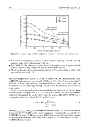
![124 HSDPA/HSUPA for UMTS
. Network algorithms – HSDPA-specific algorithms such as the MAC-hs packet
scheduler, HS-DSCH link adaptation, HS-SCCH power control and HSDPA trans-
mission resource allocation.
. Deployment scenario – the interference levels in the cell defined by factors such as
propagation loss, RF dominance areas, mobility patterns, and multipath propagation.
. UE receiver performance and capability – peak data rate, number of high-speed physical
downlink shared channel (HS-PDSCH) codes, number of transmit and receive
antennas, and baseband receiver algorithms.
. Traffic and quality of service (QoS) – mixture of Release 99 dedicated channel (DCH)
and HSDPA suitable traffic, number of active users, and their corresponding QoS
requirements.
We will attempt to adhere closely to the basic assumptions agreed in the Third
Generation Partnership Project (3GPP). During the discussion of results, it will be
indicated which factors in the above play the most important role.
7.1.1 Essential performance metrics
The fundamental features of HSDPA link adaptation functionality is adaptive modula-
tion and coding (AMC), multicode transmission (multiple HS-PDSCHs), and fast L1
hybrid automatic repeat request (HARQ). With these different domains for adaptation,
the notation for HSDPA performance evaluation is slightly different from that tradi-
tionally used for Release 99 DCHs. WCDMA Release 99 typically uses Eb =N0 to denote
the received-energy-per-user-bit-to-noise ratio. The Eb =N0 corresponds uniquely to a
certain block error rate (BLER) for a given data rate where the only adaptation param-
eter is the spreading gain. However, the Eb =N0 metric is not an attractive measure for
HSDPA because the bit rate on the HS-DSCH is varied every transmission time interval
(TTI) using different modulation schemes, effective code rates, and a number of HS-
PDSCH codes. We therefore define the average HS-DSCH signal-to-interference-plus-
noise ratio (SINR) as the narrowband SINR ratio after de-spreading the HS-PDSCH.
Referring to the notation in Figure 7.1, we can express the average HS-DSCH SINR for a
single-antenna Rake receiver as:
PHS-DSCH
SINR ¼ SF16 ð7:1Þ
ð1 À Þ Á Pown þ Pother þ Pnoise
where SF16 is the HS-PDSCH spreading factor of 16, PHS-DSCH is the received power of
the HS-DSCH summing over all active HS-PDSCH codes, Pown is the received own-cell
interference, is the downlink orthogonality factor [2]–[4], Pother is the received other-
cell interference, and Pnoise is the received noise power. In some 3GPP documents, own-
cell interference is denoted Ior while other-cell interference is expressed as Ioc . Note
from (7.1) that the HS-DSCH SINR is independent of the number of HS-PDSCH
codes used, the modulation scheme, and the effective code rate. The HS-DSCH
SINR metric is an essential measure for HSDPA link budget planning and network
dimensioning. Another commonly used and related parameter is the wideband ratio of](https://image.slidesharecdn.com/wileyhsdpahsupaforumts-12712250730845-phpapp02/85/Hsdpa-Hsupa-For-Umts-149-320.jpg)
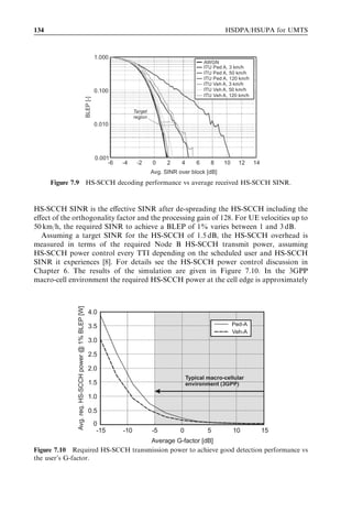
![126 HSDPA/HSUPA for UMTS
7.2.1 Basic modulation and coding performance
HSDPA provides adaptive modulation and coding to adjust the data rate to the available
channel quality. To maximize coverage and robustness, quadrature phase shift keying
(QPSK) is used together with relatively low-rate turbo-coding and a single HS-PDSCH
code. The effective code rate (ECR) can be lowered to 1/7 ¼ 137/960 meaning that 137
bits are carried using 960 channel bits per TTI per HS-PDSCH code. ECR values less
than 1/3 are achieved using repetition coding [1]. When channel conditions are better,
power can be divided among several HS-PDSCHs to ensure the most effective SINR
operating point for each code. For very high SINR conditions, 16-quadrature amplitude
modulation (16QAM) with only a little channel coding is employed. To illustrate the
dynamic range of the system, consider the example modulation and coding sets in
Table 7.1 that are called ‘transmission format and resource combinations’ (TFRCs).
The values used for TFRCs denote the signalling values of the transport block size that is
sent over the HS-SCCH. For the exact definition see [4].
The performance of the above-mentioned TFRCs has been simulated using the
following assumptions:
. A standard single antenna Rake receiver at the UE.
. The user equipment (UE) supports 5, 10, 15 HS-PDSCH codes and 16QAM.
. A Max-Log-MAP turbo-decoder using eight iterations.
. Primary common pilot channel (P-CPICH) based channel estimation is used.
. Other-cell interference is modelled using additive white Gaussian noise (AWGN).
. The default UE velocity is 3 km/h.
The link between the first transmission block error probability (BLEP) and the available
HS-DSCH SINR is shown in Figure 7.2 for a flat Rayleigh fading channel at a slow
mobile speed. Each curve relates to the TFRCs of Table 7.1 with curves to the right
Table 7.1 Example transmission format and resource combinations (TFRCs).
TFRC Modulation Effective code rate Instantaneous data rate
(ECR) with 1 HS-PDSCH code
[kbps]
000 QPSK 0.14 68.5
010 QPSK 0.27 128.5
020 QPSK 0.39 188.5
030 QPSK 0.52 248.5
040 QPSK 0.64 308.0
050 QPSK 0.77 368.5
000 16QAM 0.32 302.5
010 16QAM 0.38 362.0
020 16QAM 0.45 433.0
030 16QAM 0.54 518.0
040 16QAM 0.65 619.5
050 16QAM 0.77 741.5](https://image.slidesharecdn.com/wileyhsdpahsupaforumts-12712250730845-phpapp02/85/Hsdpa-Hsupa-For-Umts-151-320.jpg)
![HSDPA bit rates, capacity and coverage 127
1.00
BLEP
0.10
QPSK
16QAM
#20
#00 #50 #40
#10 #50
#20 #40
#00 #10 #30 #30
0.01
-8 -6 -4 -2 0 2 4 6 8 10 12 14
Instantaneous required HS-DSCH SINR [dB]
Figure 7.2 Plot of block error probability (BLEP) as a function of the instantaneous HS-DSCH
SINR. The BLEP is shown for the parameters given in Table 7.1. This simulation setup is for a
1 Â 1 RAKE receiver using an AWGN channel.
generally indicating a higher transmission data rate. There is a crossover point around
ECR ¼ 3/4 when it is beneficial to employ 16QAM with strong coding rather than using
QPSK with reduced coding.
The results presented in Figure 7.2 are for the single HS-PDSCH case showing the
basic modulation and coding performance without link adaptation. Link adaptation
selects the modulation and coding scheme so that throughput and delay are optimized for
the instantaneous SINR. Figure 7.3 shows the required SINR as a function of the data
rate for the first transmission when link adaptation is included.
AWGN, 1x1 RAKE
25
Req. HS-DSCH SINR @ 10% BLEP [dB]
10 codes
20
5 codes 15 codes
15
Dynamic
range (DR)
10
5
QPSK region
0 16QAM region
-5
0.1 1 10
Per-TTI data rate [Mbps]
Figure 7.3 Illustration of the required HS-DSCH SINR to achieve a certain first transmission
data rate with the above-mentioned TFRCs.](https://image.slidesharecdn.com/wileyhsdpahsupaforumts-12712250730845-phpapp02/85/Hsdpa-Hsupa-For-Umts-152-320.jpg)
![128 HSDPA/HSUPA for UMTS
Note the steps down at certain points in the required SINR in Figure 7.3 when
increasing the data rates, especially those between SINR 0 and 5 dB. These steps indicate
the points when the number of HS-PDSCH codes is increased from one to two, two to
three, etc.
The curves with 5, 10, and 15 codes follow each other up to approx 1 Mbps. At higher
data rates 10 and 15 codes require lower SINR than 5 codes. The reason is that 5-code
transmission has to reduce the amount of channel coding, which leads to lower spectral
efficiency than is the case when employing more HS-PDSCHs. The same is true when
comparing the curves for 10 and 15 codes for data rates above 2–3 Mbps.
Figure 7.3 also shows when QPSK or 16QAM modulation is preferred. For a low
SINR, QPSK is preferred, while for high SINR conditions, 16QAM is required to
provide the higher data rates. For 5-code transmission, 16QAM is preferred when
the instantaneous SINR is higher than approximately 10 dB.
The curves indicate that with 5 HS-PDSCH codes and 16QAM, the HS-DSCH
dynamic range equals 20 dB – that is, from À3 dB to 17 dB. Increasing the number of
HS-PDSCH codes to 15, the total dynamic range is increased to 24 dB. During HSDPA
network dimensioning it is important to set the Node B HS-DSCH transmit power such
that the HS-DSCH SINR experienced by the different users in the cell is within the HS-
DSCH dynamic range. Setting the HS-DSCH transmit power too high will result in
excessive interference in the network without achieving higher HSDPA cell throughput
if many of the users operate at the high end of the dynamic range. Similarly, if the
HS-DSCH transmit power is too low, the highest data rates cannot be achieved in the
network.
7.2.2 HS-DSCH performance
The previous section considered the performance of different modulation and coding
schemes without retransmission and without link adaptation. This section presents
HS-DSCH performance when link adaptation and retransmission schemes are included.
Figure 7.4 illustrates the HS-DSCH link level performance with 15 codes as a function
of the HS-DSCH wideband carrier-to-interference ratio (C/I). The wideband C/I is the
received power of HS-DSCH divided by noise and interference without de-spreading.
The HS-DSCH data rate is compared with the theoretical Shannon capacity for a
3.84-MHz bandwidth. The Shannon formula gives the maximum error-free data rate
that can be transmitted with a specified bandwidth in the presence of noise and inter-
ference [5]. There is only an approximate 2-dB difference between the Shannon limit
and the simulated HS-DSCH performance, mainly due to decoder limitations and
receiver estimation inaccuracies. Simulation results show that HSDPA link performance
approaches theoretical limits.
The following assumptions are used in the detailed link adaptation studies later in this
chapter:
. The HS-DSCH link adaptation algorithm in Chapter 6 is used, with both an inner
loop and an outer loop algorithm.](https://image.slidesharecdn.com/wileyhsdpahsupaforumts-12712250730845-phpapp02/85/Hsdpa-Hsupa-For-Umts-153-320.jpg)
![HSDPA bit rates, capacity and coverage 129
Supported effective data rate [Mbps]
10.0 Shannon limit:
3.84MHz*log2(1+C/I)
QPSK 16QAM
1.0
HSDPA link
adaptation curve
0.1
15 HS-PDSCH allocation
(Rake, Pedestrian-A, 3km/h)
0.01
-15 -10 -5 0 5 10 15 20
Instantaneous HS-DSCH C/I before processing gain [dB]
Figure 7.4 HSDPA data rate compared with the Shannon limit as a function of an average
HS-DSCH C/I.
. Incremental redundancy with a maximum of four transmissions. A constellation
rearrangement for 16QAM is modelled for retransmissions (the constellation re-
arrangement is discussed in Chapter 4).
. A log-normally distributed channel quality information (CQI) measurement error at
the UE with a standard deviation of 1 dB.
. The delay from CQI measurement until it is reported to the Node B and used for
adaptation is assumed to be 6 ms.
The possible inaccuracies in link adaptation are partly compensated by the use of HARQ
with soft combining, since the energy from erroneous transmissions helps to improve the
probability of correctly decoding retransmissions. The performance aspects of HARQ
have been studied in [6]. HSDPA supports both incremental redundancy as well as simple
chase combining. Incremental redundancy provides additional gain over chase combin-
ing when the effective code rate of the first transmission exceeds 1/3 [1], [6]. The typical
link adaptation target level is 10% BLER after the first transmission.
Figure 7.5 shows the single-user average throughput including link adaptation and
HARQ as a function of the average HS-DSCH SINR experienced. The results are shown
for 5, 10 and 15 codes. An average HS-DSCH SINR of 23 dB is required to achieve the
maximum data rate of 3.6 Mbps with 5 HS-PDSCH codes, and over 30 dB for 10 Mbps
with 15 codes.
The curves are very similar for different multipath profiles. Note that with a given
other-cell-to-own-cell-interference ratio, the SINR is not constant but depends on a
number of factors including orthogonality and UE receiver capabilities. These factors
must be considered when calculating the value for SINR. The benefit of SINR modelling
is that the mapping from SINR to the data rate is fairly constant for the different
environments and different UE receiver capabilities.](https://image.slidesharecdn.com/wileyhsdpahsupaforumts-12712250730845-phpapp02/85/Hsdpa-Hsupa-For-Umts-154-320.jpg)
![130 HSDPA/HSUPA for UMTS
12
5 codes, PedA
Average single-user throughput [Mbit/s]
10 5 codes VehA
5 codes fit
10 codes PedA
10 codes VehA
8
10 codes fit
15 codes PedA
15 codes VehA
6 15 codes fit
4
2
0
-10 -5 0 5 10 15 20 25 30 35 40
Average HS-DSCH SINR [dB]
Figure 7.5 HSDPA data rate as a function of average HS-DSCH SINR. Note that the effect of
link adaptation and HARQ is included in these results.
The results in Figure 7.5 can be used for HSDPA link budget planning and HSDPA
network dimensioning, since the required HS-DSCH SINR is given for different max-
imum numbers of HS-PDSCH codes and HS-DSCH throughputs. As an example, the
HSDPA single-user throughput is evaluated as a function of the path loss towards the
serving HS-DSCH cell by using the results in Figure 7.5 and the expression in Eq. (7.1).
Let’s first assume that the HSDPA user is subject only to own-cell interference and
thermal receiver noise – that is, there is no other-cell interference. Other basic assump-
tions are summarized in Table 7.2.
Given these assumptions, the HS-DSCH single-user throughput is plotted in
Figure 7.6 vs the path loss. At a path loss of 160 dB the throughput is approximately
200–400 kbps depending on HSDPA power allocation. For smaller path loss values,
Table 7.2 Basic simulation parameters used for the results
presented in Figure 7.6.
Parameter Settings
Total Node-B Tx power 12 W
Node-B cable loss 4 dB
Node-B antenna gain 18 dBi
UE antenna gain 0 dBi
UE thermal noise power À101 dBm
Allocated HS-PDSCH codes 5
Allocated HS-PDSCH power 3 or 7 W
P-CPICH Tx power 2W](https://image.slidesharecdn.com/wileyhsdpahsupaforumts-12712250730845-phpapp02/85/Hsdpa-Hsupa-For-Umts-155-320.jpg)
![HSDPA bit rates, capacity and coverage 131
10.00
Average single-user throughput [Mbit/s]
Ped-A
Veh-A
1.00 7W
HS-DSCH
power
allocation
0.10
3W HS-DSCH
power allocation
0.01
110 120 130 140 150 160 170 180
Path loss [dB]
Figure 7.6 Plot of the average single user throughput as a function of the path loss.
throughput increases. For a path loss smaller than 140 dB, HSDPA throughput is
limited by inter-path interference and is, therefore, much lower for the Vehicular A
than the Pedestrian A channel. For a 140-dB path loss in the Pedestrian A channel
profile, HSDPA throughput equals 3 Mbps, and it can be seen that, even for lower path
loss values, throughput does not increase.
Next, we consider HSDPA coverage including the effect of other-cell interference.
Assuming that the G-factor at the cell edge is known, the results in Figure 7.5 can be used
as input to dimension the required Node B HS-DSCH transmit power to guarantee a
minimum HS-DSCH throughput at the cell edge. Rearranging (7.1), we can express the
average HS-DSCH SNIR as:
PHS-DSCH 1
SINR ¼ SF16 ð7:3Þ
Pown 1 À þ G À1
and, hence, we can write:
Pown
PHS-DSCH ! SINR½1 À þ G À1 Š ð7:4Þ
SF16
where PHS-DSCH and Pown are the Node B HS-DSCH transmit power and the total
carrier transmit power, respectively. Thus, for a typical macro-cell edge with G ¼ À3 dB,
¼ 0.5, and Pown ¼ 12 W, we can calculate the minimum required HS-DSCH transmit
power to achieve a certain minimum single-user HS-DSCH data rate at the cell edge. As
an example, the HS-DSCH transmit power should equal 5.6 W if the required HS-DSCH
throughput at the cell edge needs to be 200 kbps – that is, corresponding to a required
HS-DSCH SINR of 5 dB according to Figure 7.5.
In the following we calculate the percentage of the cell area in which an HSDPA single-
user can be served with a given minimum data rate on the HS-DSCH. For these
calculations, we assume a typical macro-cellular scenario with the following parameter
settings:](https://image.slidesharecdn.com/wileyhsdpahsupaforumts-12712250730845-phpapp02/85/Hsdpa-Hsupa-For-Umts-156-320.jpg)
![132 HSDPA/HSUPA for UMTS
4.0
Average single-user throughput [Mbit/s]
Ped-A
3.5
Veh-A
3.0
2.5 3W HS-DSCH
power allocation
2.0
7W HS-DSCH
1.5 power allocation
1.0
0.5
0
0 20 40 60 80 100
Minium cell coverage area [%]
Figure 7.7 Average single-user throughput as a function of minimum cell coverage area.
. A standard homogeneous three-sector macro-cellular topology with 65 Node B
antennas and a site-to-site distance of 2.8 km.
. The COST 231 Hata Okumura path loss model is applied, plus a log-normal dis-
tributed shadow-fading component with 8-dB standard deviation.
. All cells in the network are assumed to transmit at 12 W, corresponding to a fairly high
air–interface load in all cells.
The results are plotted in Figure 7.7. Using 7 W and five HS-PDSCH codes for HSDPA,
an HSDPA single-user can be served with 1.1 Mbps in 50% of the cell area in Vehicular A
and with 1.6 Mbps in Pedestrian A. Note here that these results are obtained under the
assumption that the remaining power up to 12 W is used by Release 99 channels on the
same carrier.
Finally, a commonly used measure for network dimensioning is the pilot Ec =Io . Based
on the wideband average P-CPICH Ec =Io it is possible to estimate the achievable HSDPA
single-user throughput. It can be shown that the average HS-DSCH SINR can be
expressed as a function of the P-CPICH single Ec =Io as:
PHSDPA
SINR ¼ SF16 ð7:5Þ
Ppilot
À Pown
pilot
where PHSDPA , Pown , and Ppilot are the HSDPA transmit power, the total Node B transmit
power, and the P-CPICH transmit power, respectively. The parameter pilot denotes the
P-CPICH Ec =Io when HSDPA power is on. HSDPA single-user throughput as a function
of the average HS-DSCH SINR can be seen in Figure 7.5 for cases where 5, 10, and 15
HS-PDSCHs are available.](https://image.slidesharecdn.com/wileyhsdpahsupaforumts-12712250730845-phpapp02/85/Hsdpa-Hsupa-For-Umts-157-320.jpg)
![HSDPA bit rates, capacity and coverage 133
Table 7.3 The additional parameters used to illustrate
the impact of disabling 16QAM.
UE category Multicodes and modulation
Category 6 5-code 16QAM max 3.6 Mbps
Category 12 5-code QPSK max 1.8 Mbps
7.2.3 Impact of QPSK-only UEs in early roll-out
HSDPA UE Categories 6 and 12 both support five HS-PDSCH codes. The difference is
in the support of 16QAM modulation: Category 12 only supports QPSK modulation,
while Category 6 also supports 16QAM. The UE capabilities for Categories 6 and 12 are
summarized in Table 7.3. Single-user link performance is shown in Figure 7.8 for these
UE categories. 16QAM can clearly provide higher data rates with high SINR values
especially in the Pedestrian A channel. On the other hand, at low SINR values there is no
difference in throughput between 16QAM/QPSK and QPSK-only. For data rates lower
than 1 Mbps, performance is practically identical for the two UE categories considered.
The reason can be seen from Figure 7.3, where 16QAM is used only for higher SINR
values.
7.2.4 HS-SCCH performance
The error probability of HS-SCCH should be low since the HS-DSCH can only be
decoded by the UE if the HS-SCCH is first correctly received. Link simulation results
illustrating the HS-SCCH BLEP vs the SINR per TTI are shown in Figure 7.9. The
6 RLC PDU size=656, 5 code UE, 3 km/h
x 10
3.5
With 16QAM
QPSK-only
3
2.5
Throughput [bps]
Pedestrian A
2
Vehicular A
1.5
1
0.5
0
-10 -5 0 5 10 15 20 25 30
Average HSDPA SINR [dB]
Figure 7.8 Single-user five-code performance with 16QAM/QPSK and with QPSK-only.](https://image.slidesharecdn.com/wileyhsdpahsupaforumts-12712250730845-phpapp02/85/Hsdpa-Hsupa-For-Umts-158-320.jpg)
![134 HSDPA/HSUPA for UMTS
1.000
AWGN
ITU Ped A, 3 km/h
ITU Ped A, 50 km/h
ITU Ped A, 120 km/h
ITU Veh A, 3 km/h
0.100 ITU Veh A, 50 km/h
ITU Veh A, 120 km/h
BLEP [-]
Target
region
0.010
0.001
-6 -4 -2 0 2 4 6 8 10 12 14
Avg. SINR over block [dB]
Figure 7.9 HS-SCCH decoding performance vs average received HS-SCCH SINR.
HS-SCCH SINR is the effective SINR after de-spreading the HS-SCCH including the
effect of the orthogonality factor and the processing gain of 128. For UE velocities up to
50 km/h, the required SINR to achieve a BLEP of 1% varies between 1 and 3 dB.
Assuming a target SINR for the HS-SCCH of 1.5 dB, the HS-SCCH overhead is
measured in terms of the required Node B HS-SCCH transmit power, assuming
HS-SCCH power control every TTI depending on the scheduled user and HS-SCCH
SINR it experiences [8]. For details see the HS-SCCH power control discussion in
Chapter 6. The results of the simulation are given in Figure 7.10. In the 3GPP
macro-cell environment the required HS-SCCH power at the cell edge is approximately
Avg. req. HS-SCCH power @ 1% BLEP [W]
4.0
3.5 Ped-A
Veh-A
3.0
2.5
2.0
Typical macro-cellular
1.5 environment (3GPP)
1.0
0.5
0
-15 -10 -5 0 5 10 15
Average G-factor [dB]
Figure 7.10 Required HS-SCCH transmission power to achieve good detection performance vs
the user’s G-factor.](https://image.slidesharecdn.com/wileyhsdpahsupaforumts-12712250730845-phpapp02/85/Hsdpa-Hsupa-For-Umts-159-320.jpg)
![HSDPA bit rates, capacity and coverage 135
0.5 W and on average is 0.2–0.3 W over the cell area, which is 2% of average Node B
transmission power. These simulations assume round robin scheduling, which does not
take the current radio channel conditions into account. The impact of more advanced
scheduling on the HS-SCCH overhead has been studied in [7]. When scheduling the
data – primarily when the user’s channel is favourable – a side-benefit is that the
HS-SCCH overhead is reduced.
Each code-multiplexed user requires an HS-SCCH. If we code-multiplex three users,
three parallel HS-SCCHs are required. Therefore, the optimization of HS-SCCH power
control becomes more relevant when code-multiplexing is used.
More detailed design considerations and performance figures for the HS-SCCH can
be found in [10].
7.2.5 Uplink HS-DPCCH performance
The uplink HS-DPCCH is power-controlled relative to the uplink DPCCH in every slot
interval. The power relation between the DPCCH and the HS-DPCCH is given by the
parameters [DACK ; DNACK ; DCQI ], which are set by the radio network controller (RNC)
via radio resource control (RRC) signalling to the UE. The power offset can be up to 6 dB
within nine possible quantization steps [14]. The power offsets [DACK ; DNACK ; DCQI ] must
be selected to fulfill the required uplink HS-DPCCH detection probabilities. The normal
target values for these offsets are defined in terms of the probability of mis-detecting.
Typical values for these are PACK ! NACK 10 À2 and PNACK ! ACK 10 À3 . The prob-
ability of decoding a NACK as an ACK has to be very low since that causes missing L1
retransmission and the data must be retransmitted by the RLC layer.
In a previous study [13], the default values for HS-DPCCH power offsets have been
extracted that fulfill the HS-DPCCH detection probabilities as specified by 3GPP. It
should be noted that the recommended default HS-DPCCH power offsets depend on
the service on the uplink-associated DCH. The DPCCH/DPDCH power offset is set to
À2.69 dB for the 12-kbps service [32]. The recommended values are [13]: DACK ¼ 4 dB,
DNACK ¼ 4 dB, and DCQI ¼ 2 dB. With an increasing data rate on the DCH, the above
offsets generally decrease.
These numbers are valid for HSDPA users with an active set size of 1. The uplink
power control in soft handover is based on the best uplink connection – that is, if one
of the cells receives a high enough signal level, mobile power can be decreased. The
HS-DPCCH, however, is received only by the serving HS-DSCH cell and the received
power level of the HS-DPCCH may be too low if that cell instantaneously does not have
the best uplink connection. Therefore, a larger HS-DPCCH power offset is required
in soft handover. If the maximum power offset of 6 dB is not enough to maintain
HS-DPCCH quality, 3GPP specifications allow the use of ACK/NACK repetition as
well. For HSDPA users in soft handover, it is recommended to use an HS-DPCCH
power offset of 6 dB and an ACK/NACK repetition of 2 resulting in an additional gain
of approximately 3 dB. For further information on HS-DPCCH uplink coverage for
users in soft handover, the reader is referred to [13].](https://image.slidesharecdn.com/wileyhsdpahsupaforumts-12712250730845-phpapp02/85/Hsdpa-Hsupa-For-Umts-160-320.jpg)
![136 HSDPA/HSUPA for UMTS
7.2.6 3GPP test methodology
HSDPA performance requirements are defined in [11]. In this text, the focus is on the
single link performance of the HS-DSCH with a constant modulation and coding
scheme. For the simulations shown here, it has been assumed that the return channel
for HSDPA (HS-DPCCH) is error-free when transmitting ACKs/NACKs in response
to a HARQ.
In [11], various test channels are defined – denoted as H-Set1 to H-Set6 – each
describing different UE capabilities. These channels are called ‘fixed reference channels’
(FRCs). Here, we will only consider the first test channel (H-Set1). The test channel
definitions are shown in Table 7.4. The minimum performance requirements for QPSK
and 16QAM are listed in Tables 7.5 and 7.6, respectively. QPSK modulation is tested
with own-to-other-cell-interference ratio Ior =Ioc values of 0 dB and 10 dB. The value of
0 dB corresponds to a location close to the cell edge while 10 dB is located in a clear
dominance area of a single cell. 16QAM modulation is tested only with an own-to-other-
cell-interference ratio of 10 dB since 16QAM would not be used at a low Ior =Ioc value.
Two HS-DSCH power allocations are considered: 25% of Node B power for HS-DSCH
(Ec =Ior ¼ À6 dB) and 50% power for HS-DSCH (Ec =Ior ¼ À3 dB).
We compare the link simulations with the 3GPP minimum performance requirements
given in Figure 7.11 as a function of HS-DSCH power allocation. ITU Vehicular A
multipath profile at 30 km/h is assumed in Figure 7.11. The simulated results are
Table 7.4 Parameter settings for simulation of the fixed reference channel H-Set1.
Parameter Unit Value
Modulation QPSK 16QAM
Inter-TTI distance TTI’s 3 TTI 3 TTI
Effective code rate 0.67 0.61
Number of physical channel codes Codes 5 4
Table 7.5 Minimum requirement QPSK, fixed reference channel (FRC) H-Set1.
Test Propagation Reference value
number conditions
HS-PDSCH Ec =Ior Data rate at Data rate at
Ior =Ioc ¼ 0 dB Ior =Ioc ¼ 10 dB
[dB] [kbps] [kbps]
1 Pedestrian A À6 65 309
3 km/h À3 N/A 423
2 Pedestrian B À6 23 181
3 km/h À3 138 287
3 Vehicular A À6 22 190
30 km/h À3 142 295
4 Vehicular A À6 13 181
120 km/h À3 140 275](https://image.slidesharecdn.com/wileyhsdpahsupaforumts-12712250730845-phpapp02/85/Hsdpa-Hsupa-For-Umts-161-320.jpg)
![HSDPA bit rates, capacity and coverage 137
Table 7.6 Minimum requirement 16QAM, fixed reference channel (FRC) H-Set1.
Test number Propagation Reference value
conditions
HS-PDSCH Data rate at
Ec =Ior Ior =Ioc ¼ 10 dB
[dB] [kbps]
1 Pedestrian A À6 198
3 km/h À3 368
2 Pedestrian B À6 34
3 km/h À3 219
3 Vehicular A À6 47
30 km/h À3 214
4 Vehicular A À6 28
120 km/h À3 167
Channel profile: Vehicular A, 30 km/h, Set1
500
G factor=10 dB, simulations
450 G factor=10 dB, requirement
G factor=10 dB, 16QAM, simulations
400 G factor=10 dB, 16QAM, requirement
G factor=0 dB, simulations
350 G factor=0 dB, requirement
Throughput [kbps]
300
250
200
150
100
50
0
-12 -11 -10 -9 -8 -7 -6 -5 -4 -3 -2
Allocated HS-DSCH power [dB]
Figure 7.11 Throughput performance of H-Set1 as a function of allocated HS-DSCH power for
the Vehicular A 30 km/h channel profile.
approximately 1–2 dB better than 3GPP performance requirements. The results pre-
sented in Figure 7.11 can be viewed as either a margin in terms of throughput or as an
implementation margin.
7.3 Multiuser system performance
The following subsections contain multiuser simulation results. We provide both cell
capacity and end user performance results. Most of the results are obtained for best](https://image.slidesharecdn.com/wileyhsdpahsupaforumts-12712250730845-phpapp02/85/Hsdpa-Hsupa-For-Umts-162-320.jpg)
![138 HSDPA/HSUPA for UMTS
effort web browsing applications without any strict QoS requirements. Some results for
constant bit rate streaming applications are also presented.
7.3.1 Simulation methodology
The performance of HSDPA in a multiuser scenario is quantified by conducting
advanced dynamic network level simulations with multiple cells and users [8]. The
simulator supports scenarios with a mixture of WCDMA Release 99 DCH and
HSDPA Release 5 users being served by the same carrier. For each Release
5 HSDPA user, we explicitly simulate reception of HS-DSCH, HS-SCCH, and one
associated DCH at 3.4 kbps. The associated DCH is only assumed to carry the signalling
radio bearer for Layer 3 signalling. Release 99 DCHs are simulated with inner loop and
outer loop power control, soft handover functionality, and power-based admission
control. The primary default simulation parameters are summarized in Table 7.7 [8].
7.3.2 Multiuser diversity gain
We first study the gain of proportional fair scheduling over round robin, also called
‘multiuser diversity gain’. Multiuser diversity gain is reported in Figure 7.12 for the case
where 7 W and five HS-PDSCH codes are allocated for HSDPA transmission, while the
remaining available resources are used for transmission of Release 99 channels [8]. The
average number of HSDPA users per cell equals six for these results. Multiuser diversity
gain comes from scheduling users when they experience relatively good SINR, while
avoiding scheduling users that experience deep fades. Multiuser diversity gain is only
available at moderate UE speeds where the packet scheduler is able to track fast fading
radio channel variations. At high UE speeds where the packet scheduler can no longer
track radio channel variations by monitoring received CQI reports from UEs, multiuser
diversity gain is marginal. The same observation is true for stationary users where the
channel is constant. The proportional fair scheduler can provide a minor gain at 0 km/h
Table 7.7 Summary of default parameter settings for network simulations.
Network topology Macro-cellular, three-sector sites, 2.8-km site-to-site distance
Radio propagation COST231 Okumura–Hata, log-normal shadowing (8 dB std), ITU
Vehicular A with 3 km/h.
MAC-hs functionalities Proportional fair packet scheduling, HARQ with chase combining.
Traffic model Closed loop TCP web browsing model, 1500 bytes TCP packet size,
100 kbytes average packet call size, RLC acknowledged mode.
Handovers Synchronized HS-DSCH cell change for HSDPA, standard soft
handover for Release 99 with an add window of 2 dB.
UE receiver type Single antenna Rake.
Node B power settings Maximum transmit power per cell 20 W, P-CPICH power 2 W.](https://image.slidesharecdn.com/wileyhsdpahsupaforumts-12712250730845-phpapp02/85/Hsdpa-Hsupa-For-Umts-163-320.jpg)
![HSDPA bit rates, capacity and coverage 139
40
35
Multi-user diversity gain [%]
30
25
20
15
10
5
0
0 5 10 15 20 25 30 35 40 45 50
UE Speed [kmph]
Figure 7.12 Multiuser diversity gain as a function of the UE speed.
as well due to variations in the interference. The results in Figure 7.12 are obtained for a
Vehicular A radio channel.
Multiuser diversity gain also depends on the number of simultaneous active HSDPA
users in the cell. The gain of proportional fair over round robin is reported in Figure 7.13
vs the number of HSDPA users, assuming that all users are moving with a velocity of
3 km/h. A clear gain can already be achieved with two parallel users. Multiuser diversity
gain only increases marginally as the number of users goes beyond five. It is also observed
60
50
Pedestrian A
Multi-user diversity gain [%]
40
30
Vehicular A
20
10
0
1 2 3 4 5 6
Number of HSDPA users
Figure 7.13 Multiuser diversity gain as a function of number of HSDPA users at 3 km/h.](https://image.slidesharecdn.com/wileyhsdpahsupaforumts-12712250730845-phpapp02/85/Hsdpa-Hsupa-For-Umts-164-320.jpg)
![140 HSDPA/HSUPA for UMTS
that multiuser diversity gain is larger in International Telecommunication Union (ITU)
Pedestrian A than in ITU Vehicular A. This behaviour is due to the larger fading
dynamic range in ITU Pedestrian A. Recall that multiuser diversity gain increases
when the fading dynamic range of the radio channel increases. Additional simulation
results for ITU Pedestrian A are shown in Section 7.7.3.6.1.
7.3.3 HSDPA-only carrier capacity
Cell throughput results are reported in Figure 7.14 for different allocations of
HS-PDSCH codes per cell in an ITU Vehicular A multipath. For five HS-PDSCH
codes and no DCH traffic in the cell, achievable cell throughput is found to equal
1.2 Mbps, while it increases to 1.3 Mbps if some of the power is also used for transmission
of traffic on the DCH. Hence, with five HS-PDSCH codes per cell, it is better to split the
traffic between HSDPA and the DCH rather than allocating all the traffic and power to
HSDPA. The practical split between HSDPA and the DCH obviously depends on the
available traffic from HSDPA and non-HSDPA UEs. Increasing the number of
HS-PDSCH codes from five to ten results in a capacity gain of approximately 50%.
The capacity increase is achieved because it is more spectrally efficient to first increase the
number of HS-PDSCH codes before starting to increase the effective coding rate and/or
modulation order. The results for ten HS-PDSCH codes in an HSDPA-only cell are
reported for the case without code-multiplexing assuming that all HSDPA mobiles are
able to receive up to ten HS-PDSCH codes and with code-multiplexing of two users per
TTI, each capable of receiving five HS-PDSCH codes. It is observed that achievable
2.5
Code-mux with 5 code UEs
No code-mux (no UE code limitations)
2.0
Average cell throughput [Mbps]
1.5
1.0
DCH+HSDPA
HSDPA only
HSDPA only
HSDPA only
HSDPA only
HSDPA only
0.5
0.0
5 codes 10 codes 15 codes
Available number of HS-PDSCH codes per cell
Figure 7.14 Average cell throughput as a function of allocated number of HS-PDSCH codes and
whether code-multiplexing used.](https://image.slidesharecdn.com/wileyhsdpahsupaforumts-12712250730845-phpapp02/85/Hsdpa-Hsupa-For-Umts-165-320.jpg)
![HSDPA bit rates, capacity and coverage 141
cell throughput is slightly lower in the case of code-multiplexing. This is caused by the
higher overhead from having two HS-SCCHs per cell as well as the additional scheduling
constraints from having to schedule two users per TTI. The cell capacity with all 15 codes
is approximately 2.0 Mbps when code-multiplexing is used.
7.3.4 HSDPA capacity with Release 99
We consider the case where five HS-PDSCH codes and one HS-SCCH code are allocated
for HSDPA transmission per cell. This can be considered a typical initial roll-out
scenario for HSDPA. The remaining channelization codes are used for the transmission
of Release 99 channels. Figure 7.15 shows the average cell throughput on HSDPA and
the DCH vs the allocated HSDPA power, as well as the total cell throughput that
is the sum of the throughput on HSDPA and the DCH. As expected, HSDPA cell
throughput increases the more HSDPA power that is being allocated, while DCH
throughput simultaneously decreases. The maximum cell throughput is observed to
equal 1.3 Mbps for 7-W HSDPA power allocation. Hence, the introduction of
HSDPA with five HS-PDSCH codes brings a capacity gain of 70% over Release 99,
which typically offers a capacity of 780 kbps. The capacity gain comes from fast link
adaptation and HARQ, and multiuser diversity comes from using proportional fair
scheduling. Hence, it is evident that the performance of HSDPA vs DCH depends on
how the common transmission resources are shared between these two channel types.
However, total cell throughput does not vary significantly with HSDPA transmit power
allocated.
1400
Total throughput
1200
Cell throughput [kbps]
1000
HSDPA throughput
800
600
DCH throughput
400
200
3 4 5 6 7 8 9
Allocated HSDPA Power [W]
Figure 7.15 Average cell throughput as a function of allocated HSDPA power per cell.](https://image.slidesharecdn.com/wileyhsdpahsupaforumts-12712250730845-phpapp02/85/Hsdpa-Hsupa-For-Umts-166-320.jpg)
![142 HSDPA/HSUPA for UMTS
1.0
3 HSDPA users
0.9 on average
0.8
0.7
Cumulative distribution
0.6
5 HSDPA users
0.5 on average
1 HSDPA user
on average
0.4
0.3
0.2
0.1
0.0
0 100 200 300 400 500 600 700 800 900 1000
Per HSDPA user throughput [kbps]
Figure 7.16 Cumulative distribution function of HSDPA throughput experienced per user for
different numbers of HSDPA users per cell. The HSDPA power allocated equals 7 W.
7.3.5 User data rates
HSDPA throughput experienced per user depends on the number of allocated HSDPA
users per cell that are sharing the common HS-DSCH. The cumulative distribution
function of the HSDPA throughput experienced per user is reported in Figure 7.16,
assuming 7-W HSDPA power allocation and five HS-PDSCH codes, while the remaining
power is used for transmission of Release 99 channels. As expected, HSDPA throughput
decreases as more users are allocated per cell. The decrease in average HSDPA through-
put per user is not inversely proportional to the number of allocated HSDPA users. As an
example, HSDPA user throughput at the 50% quantile equals 400 kbps and 270 kbps for
one and three HSDPA users per cell, respectively. The reason for this is that multiuser
diversity gain increases with more users. Users experiencing high data rates are typically
close to the serving HS-DSCH cell, while users served with lower data rates are typically
at the cell edge. Although not shown here, HSDPA throughput experienced per user is
also observed to depend significantly on the amount of allocated HSDPA transmission
power, as was also observed in Figure 7.15 for average HSDPA cell throughput.
7.3.6 Impact of deployment environment
Recall that the network performance results presented have been obtained from a large
macro-cellular scenario with an ITU Vehicular A power delay profile. In the following,
we give a brief discussion on how performance results will change if some of the essential
simulation parameters are altered.](https://image.slidesharecdn.com/wileyhsdpahsupaforumts-12712250730845-phpapp02/85/Hsdpa-Hsupa-For-Umts-167-320.jpg)
![HSDPA bit rates, capacity and coverage 143
7.3.6.1 Multipath profile
It is known from the numerous radio channel measurement campaigns reported in
[25] that the ITU Vehicular A power delay profile is representative for macro-cells
where Node B antennas are mounted above the rooftop level. However, users located
in close vicinity of the Node B might experience a power delay profile with less temporal
dispersion – such as the ITU Pedestrian A channel profile (see, e.g., Greenstein’s
distance-dependent models for delay spread [24]). The ITU Pedestrian A power delay
profile is typically used for micro-cells where the Node B antenna is mounted below
rooftop level. ITU Pedestrian A has less temporal dispersion, and therefore also a better
downlink orthogonality factor [2], which results in less own-cell interference at the UE
after de-spreading. The ITU Pedestrian A channel profile also has a larger fading
dynamic range which results in larger multiuser diversity scheduling gain (see [7]).
Figure 7.17 compares both Vehicular A and Pedestrian A in a three-sector macro-
cell environment. Hence, for the macro-cellular setup under consideration, average
HSDPA cell throughput is increased by 30–50% in ITU Pedestrian A compared with
Vehicular A. Note that the use of performance enhancement methods – like the advanced
receivers in Section 7.8 – offer further improved cell throughputs over the numbers
shown in Figure 7.17.
3.5
ITU Vehicular A ITU Pedestrian A
3.0
2.5
HSDPA cell throughput [Mbps]
2.0
1.5
1.0
0.5
0.0
5 codes 10 codes 15 codes 5 codes 10 codes 15 codes
Figure 7.17 Summary of average cell throughput for HSDPA in a macro-cellular environment
depending on the assumed power delay profile and number of HS-PDSCH codes allocated.](https://image.slidesharecdn.com/wileyhsdpahsupaforumts-12712250730845-phpapp02/85/Hsdpa-Hsupa-For-Umts-168-320.jpg)
![144 HSDPA/HSUPA for UMTS
7.3.6.2 Cell topology
Cell topology does impact HSDPA performance. As an example, the results for micro-
cells have been presented [1]. The micro-cellular setup is characterized by the higher
isolation between neighbouring cells which results in less other-cell interference as well as
less multipath propagation. The average HSDPA cell throughput is therefore found to
increase from 2.2 Mbps for macro-cells to 4.8 Mbps for micro-cells. The larger HSDPA
cell throughput in micro-cells is achievable because the HS-DSCH SINR at many of the
users is sufficiently high to allow frequent transmission using 16QAM modulation.
7.3.6.3 Indoor coverage
The other simulation results in this chapter have been obtained using an urban macro-
cellular propagation model assuming users located outdoors at street level. Since quite a
few users are located indoors in practice, the earlier simulations have been repeated with
an additional indoor penetration loss of 20 dB. However, note that this additional path
loss might be too pessimistic for users located on higher floors in high-rise buildings, since
the path loss is typically observed to be less for elevated users [25], [26]. The added
penetration loss of 20 dB tends to make thermal noise at users at the cell edge dominant
over other-cell interference and, therefore, results in capacity loss when compared with
the results for the outdoor-to-outdoor situation. For the scenario under consideration –
with a 2.8-km site-to-site distance – the 20-dB penetration loss results in a 15%
throughput decrease for HSDPA. However, the throughput decrease for Release 99 is
observed to equal 40%. This clearly demonstrates that HSDPA provides an additional
coverage gain over Release 99. Using HARQ with soft combining of retransmissions and
fast scheduling mainly facilitates this coverage gain.
A dedicated indoor in-building system can also be used to significantly improve indoor
coverage – that is, using distributed antenna systems or an indoor pico-cell. As studied in
[16], HSDPA is very attractive for such scenarios since HS-DSCH SINR values are high
and 16QAM modulation can frequently be used to offer high user data rates and cell
capacities.
7.3.6.4 Estimation of HSDPA bit rates based on a WCDMA drive test
This section illustrates a method of estimating HSDPA bit rates based on WCDMA
drive test measurements. Drive tests typically provide at least CPICH Ec =N0 and CPICH
received signal code power (RSCP) measurements. Once we combine those measure-
ments with the expected power allocations for HSDPA, we can predict the HS-DSCH
SINR. Using the results of link level simulations, SINR values can be mapped to an
HSDPA bit rate. The method is illustrated in Figure 7.18. We present an example case
study from a commercial European WCDMA network.
We consider two cases for HSDPA deployment: an HSDPA-only carrier and a shared
carrier with WCDMA. Assumed power allocations are shown in Figure 7.19. The shared
carrier assumes HS-DSCH power of 7 W and the dedicated carrier 15 W. The network
load was low during the measurements and average Node B transmission power was](https://image.slidesharecdn.com/wileyhsdpahsupaforumts-12712250730845-phpapp02/85/Hsdpa-Hsupa-For-Umts-169-320.jpg)
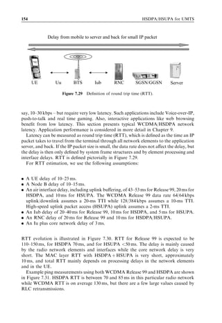
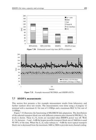
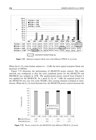
![148 HSDPA/HSUPA for UMTS
2500
2000
1500
kbps
1000
500
0
HSDPA-only 15-code Shared (7 W) 10-code Shared (7 W) 5-code
Figure 7.23 Average HSDPA bit rates with dedicated HSDPA carrier and with shared carrier.
1740 kbps for 10-code, and 2040 kbps for 15-code HSDPA. A total of 90% of the drive
test locations would provide at least 500–600 kbps.
Figure 7.23 illustrates the average bit rates achievable using dedicated and shared
carriers. A dedicated 15-code HSDPA carrier can increase throughput by 50% compared
with a 10-code HSDPA shared carrier and over 100% compared with a 5-code HSDPA
shared carrier.
This section has shown that simple measurements from an operator’s WCDMA
network can be used to obtain quick estimates of the HSDPA data rates expected in
that network.
7.3.7 HSDPA capacity for real time streaming
In the previous sections, we presented performance results for best-effort traffic without
any strict QoS constraints. In this section, we present results for constant bit rate
streaming with a play-out buffer of 5 sec. These results are obtained using the simulation
methodology and scenario described in Section 7.7.3.1, assuming that all traffic in the cell
is transmitted on the HS-DSCH with up to ten HS-PDSCH codes. For additional details
see [18].
Constant bit rate streaming services at 128 kbps are simulated using radio link control
(RLC) acknowledged mode. New streaming calls are generated according to a homo-
geneous Poisson process with a call length of 40 sec. The play-out buffer functionality at
the user is explicitly simulated. Once the amount of buffered data reaches 640 kilobits in
the play-out buffer, play-out at 128 kbps is started. Hence, with a source bit rate of
128 kbps the minimum initial buffering time equals 5 sec. If it happens that the play-out
buffer runs empty during a streaming call, then a re-buffering event occurs, where the
play-out is stopped until the buffer reaches 640 kilobits. A satisfied user is defined as a
user with an initial buffering time of less than 8 sec without experiencing any re-buffering
events. An unhappy user is a user with either an initial buffering time longer than 8 sec, or](https://image.slidesharecdn.com/wileyhsdpahsupaforumts-12712250730845-phpapp02/85/Hsdpa-Hsupa-For-Umts-173-320.jpg)
![HSDPA bit rates, capacity and coverage 149
14
Constant bit rate streaming @ 128 kbps
12
Unsatisfied user probability [%]
10
8
6
4
2
0
0.9 1.0 1.1 1.2 1.3 1.4 1.5
Average HS-DSCH cell throughput [Mbps]
Figure 7.24 Unsatisfied user probability for streaming at 128 kbps as a function of carried
HS-DSCH throughput.
a user who experiences re-buffering events. Finally, users subject to initial buffering times
or re-buffering times longer than 10 sec are dropped. Unsatisfied users are the sum of
dropped and unhappy users. These QoS definitions for streaming services are similar to
the ones used in [17]. Given these requirements for constant bit rate streaming, quality-
based HSDPA admission control may be needed if there are too many streaming users
entering the cell. Such algorithms are studied in [18] and [19]. The quality-based HSDPA
access algorithm proposed in [18] is used for the results presented in Figure 7.24, where
unsatisfied user probability is plotted vs carried HS-DSCH cell throughput. These
results are obtained by running a series of simulations with different QoS targets for
the quality-based HSDPA access algorithm. Assuming a maximum allowed unsatisfied
user probability of 5%, HSDPA cell capacity at 128-kbps streaming equals approxi-
mately 1.3 Mbps, or equivalently ten users per cell.
Advanced streaming clients and servers are able to adapt their data rate to the
available radio bit rate. Those adaptive streaming codecs are considered in Chapter 9.
7.4 Iub transmission efficiency
One of the significant operational expenses for many WCDMA operators is Iub trans-
mission between the RNC and Node Bs, especially if leased E1/T1 lines are used. This
section shows how HSDPA technology can improve Iub transmission efficiency and help
reduce the cost per transmitted bit on HSDPA compared with that on WCDMA. Today,
the majority of operators use asynchronous transfer mode (ATM) transmission on the](https://image.slidesharecdn.com/wileyhsdpahsupaforumts-12712250730845-phpapp02/85/Hsdpa-Hsupa-For-Umts-174-320.jpg)
![150 HSDPA/HSUPA for UMTS
Iub, so this will be our working assumption for the subsequent analysis, even though
Internet Protocol (IP) based transmission is also supported by 3GPP specifications. The
improved Iub efficiency for HSDPA comes from the following factors [37]:
. Fast dynamic sharing of the HSDPA Iub bandwidth allocated between active HSDPA
users. This is achieved by using fast MAC-hs flow control. With Release 99 the Iub
bandwidth is typically allocated separately per user, which makes it difficult to
dynamically share excess capacity during periods with low activity – for example,
during short reading times for web browsing applications.
. Buffering of data in the Node B means that transmission with high peak data rates at
the air interface can be supported with HSDPA without requiring a similar higher Iub
bandwidth. It also implies that short temporary periods with Iub congestion do not
necessarily result in unused HSDPA air interface capacity.
. HSDPA does not need soft handover, so the data transmitted to one HSDPA user is
only sent once over a single Iub. WCDMA Release 99 relies on soft handover, where
multiple Iub links are required for users in soft handover. As an example, results from
[13] show that the soft handover overhead equals approximately 40% for WCDMA
users, meaning that on average a Release 99 UE receives data from 1.4 cells.
Assuming a standard closed loop Transmission Control Protocol (TCP) web browsing
traffic model and a three-sector macro-cell environment, it is reported in [37] that Iub
efficiency is improved by a factor of 2 for HSDPA compared with that for WCDMA.
This is a significant improvement, which basically means that twice as many user bits can
be transmitted through the same Iub with HSDPA compared with using Release 99
WCDMA. In order to further address Iub dimensioning for HSDPA, the simulations
from Section 7.7.3.4 are repeated using Iub bandwidth restrictions and high-speed fast
medium access control (MAC-hs) flow control as illustrated in Figure 7.25. Recall from
Iub interface
RNC limited Node-B
bandwidth
MAC-d entity, User #1 MAC-hs buffer, User #1
MAC-d entity, User #2 MUX MAC-hs buffer, User #2
DEMUX MAC-hs
MAC-d entity, User #3 RNC MAC-hs buffer, User #3 packet
control scheduler
point
............
............
MAC-d entity, User #
N MAC-hs buffer, User N
#
............ Buffer information
MAC-hs flow control
6LJQDO how much data
Tell KRZ PXFK GDWD
HDFK 0$G IORZ LV
each MAC-d flow is
DOORZHG WR VHQG RYHU
allowed to send over
WKH ,XE
the Iub
Figure 7.25 Block diagram for simulation setup with limited Iub bandwidth and MAC-hs flow
control.](https://image.slidesharecdn.com/wileyhsdpahsupaforumts-12712250730845-phpapp02/85/Hsdpa-Hsupa-For-Umts-175-320.jpg)
![HSDPA bit rates, capacity and coverage 151
100 %
95 %
90 %
RF utilization [%]
85 %
Iub utilization [%]
80 %
75 %
70 %
65 %
60 %
2.0 2.2 2.4 2.6 2.8 3.0 3.2 3.4 3.6 3.8
Iub capacity for 1+1+1 site [Mbps]
Figure 7.26 Trade-off between HSDPA RF vs Iub efficiency.
Chapter 3 that MAC-hs flow control is operated by sending so-called credits to the RNC
for each MAC-d flow, depending on the amount of buffered data in the Node B. The
number of credits expresses the maximum number of payload data units (PDUs) that the
RNC is allowed to send over the Iub during the next HS-DSCH interval of 10 ms. Note
that the frame-length for the HS-DSCH frame protocol equals 10 ms. If Iub congestion
occurs so the RNC cannot transmit all the PDUs according to the received credits, a
simple congestion control scheme is applied, where the PDU flow is reduced equally for
all active HSDPA MAC-d flows.
The trade-off between air interface RF vs Iub efficiency is reported in Figure 7.26. Note
from Section 7.7.3.4 that without any Iub bandwidth limitations the average HSDPA
cell capacity equals approximately 900 kbps, which is 2.7 Mbps per three-sector Node B
assuming five HS-PDSCH codes and 7 W for HSDPA transmission. The remaining
power and some channelization codes are used for simultaneous Release 99 transmission.
The results in Figure 7.26 show that in order to achieve the full 100% HSDPA radio
frequency (RF) capacity the HSDPA Iub bandwidth required equals 3.8 Mbps. An
HSDPA Iub bandwidth of 3.2 Mbps is sufficient to achieve 95% of the maximum
available HSDPA RF capacity. Such Iub dimensioning corresponds to 20% over-
dimensioning of the Iub. This 20% over-dimensioning is needed to account for
temporal variations in the available HSDPA RF capacity caused by, for example,
HSDPA users being close to the serving cell and variations in the traffic model. Note
that the resulting 20% margin will be reduced when the number of active HSDPA users
per site is increased in high-capacity sites. In that case the peak site capacity will be closer
to the average site capacity due to the smaller dominance of a few users in extreme
conditions.
7.5 Capacity and cost of data delivery
The previous sections presented total cell throughput in Mbps, but this section estimates
the achievable data capacity in total downloaded gigabytes per subscriber per month.](https://image.slidesharecdn.com/wileyhsdpahsupaforumts-12712250730845-phpapp02/85/Hsdpa-Hsupa-For-Umts-176-320.jpg)
![152 HSDPA/HSUPA for UMTS
Data capacity depends on a number of assumptions in addition to the traffic models:
What is the ‘burstiness’ of the data transmission and how is the traffic distributed over the
day. Voice traffic tends to be relatively constant over the day and the busy hour may carry
even less than 10% of the total daily traffic. The data part depends clearly on the
applications used, but it could be more bursty, especially if HSDPA is used for fixed
wireless access from homes. We assume in the following calculations that the busy hour
carries 20% of the daily traffic. The following additional assumptions have been used in
HSDPA capacity calculation:
. A 2 þ 2 þ 2 HSDPA configuration.
. Spectral efficiency of 2 Mbps/cell using an HSDPA terminal with single antenna and
Rake receiver (see Figure 7.14).
. Spectral efficiency of 4 Mbps/cell using an HSDPA terminal with antenna diversity
and equalizer receiver (see Figure 7.38).
. Busy hour utilization 80%.
. Busy hour share of the daily traffic is 20%.
These assumptions are applied to calculate the total traffic in GB per month as follows:
2 Mbps 3600 s
ð2 þ 2 þ 2Þ Á Á 80% Á 30 days
Capacity [GB/month] ¼ 8 hour ð7:11Þ
20% busy hour share
Total carried traffic is 650 GB with a single-Rake HSDPA terminal and 1170 GB with
a two-equalizer HSDPA terminal per month per site. Figure 7.27 illustrates the
maximum HSDPA capacity per subscriber per month. These results show that a
2–4-GB/subscriber/month capacity is feasible with 300 broadband subscribers per site.
14.0
2-Equalizer
12.0
1-Rake
10.0
GB/sub/month
8.0
6.0
4.0
2.0
0.0
100 150 200 250 300 350 400 450 500 550 600
Broadband subscribers per site
Figure 7.27 Data capacity per subscriber per month.](https://image.slidesharecdn.com/wileyhsdpahsupaforumts-12712250730845-phpapp02/85/Hsdpa-Hsupa-For-Umts-177-320.jpg)
![HSDPA bit rates, capacity and coverage 153
4.0
3.5
3.0
Cost per GB [€]
2.5
2.0
1.5
1.0
0.5
0.0
10 12 14 16 18 20 22 24 26 28 30
Price per sector per carrier [k€]
Figure 7.28 Delivery cost of downloaded GB.
Another challenge – besides radio capacity – is the cost of data delivery for high-
volume data. We give below a simplified view of the cost in which only depreciation of the
network equipment capital expenditure is considered over 6 years. The cost of GB
delivery is shown as a function of network equipment price. The price in Figure 7.28
is shown per sector per carrier including base station, RNC, and core network elements.
The following formula is used to calculate the cost:
c
¼ TRX price  10 9
Cost ¼ ð7:12Þ
GB 2Mbps 80%
 3600   365  6 years
8 20%
c
If network pricing is below ¼ 16 000 per sector per carrier, the data delivery cost with
c
HSDPA is below ¼ 2/GB. That number can be considered as the lower bound of delivery
cost when new capacity is added to the system. The busy hour utilization of 80% cannot
be achieved in practice in all cells since the network must be designed to provide coverage
also in those areas where the traffic density is not as high. If the average busy hour
network utilization is 40% instead of 80%, the delivery cost is double that shown in
Figure 7.28.
This calculation excludes such cost factors as Iub transmission cost or other network
operation costs, marketing, and customer acquisition.
7.6 Round trip time
While the maximum data rate is typically used to benchmark radio systems, it is not a
sufficient measure alone to describe radio performance from the application point of
view. The pure data rate is relevant if we consider the download time of a large file,
but there are a number of applications that are happy with a relatively low data rate –](https://image.slidesharecdn.com/wileyhsdpahsupaforumts-12712250730845-phpapp02/85/Hsdpa-Hsupa-For-Umts-178-320.jpg)
![HSDPA bit rates, capacity and coverage 155
200
Iu + core
180
RNC
160 Iub
140 Node B
120 Air interface
[ms]
100 UE
80
60
40
20
0
R99 (64/64) R99 (128/384) HSDPA HSUPA (2-ms)
Figure 7.30 Estimated round trip time (RTT) evolution.
200
180
160
140
120
[ms]
100
80
60
40
WCDMA (128/384 kbps)
20 HSDPA (384 kbps/1.8 Mbps)
0
1 101
Samples
Figure 7.31 Example measured WCDMA and HSDPA RTTs.
7.7 HSDPA measurements
This section first presents a few example measurement results from laboratory and
further outdoor drive test results. The measurements were done using a Category 12
terminal with a maximum L1 bit rate of 1.8 Mbps and a maximum RLC L2 bit rate of
1.6 Mbps.
Figure 7.32 illustrates the functioning of HS-DSCH link adaptation. The distribution
of the selected transport block size with different common pilot channel (CPICH) Ec =N0
levels is shown. These Ec =N0 levels are recorded when HSDPA power was off. With
Ec =N0 between À3 and À6 dB the largest possible transport block size of 3440 bits is used
94–99% of the time. When the Ec =I0 value reduces to À9 dB the most typical transport
block size is decreased from the maximum 3440 to 2404 to provide more channel coding.](https://image.slidesharecdn.com/wileyhsdpahsupaforumts-12712250730845-phpapp02/85/Hsdpa-Hsupa-For-Umts-180-320.jpg)
![156 HSDPA/HSUPA for UMTS
Figure 7.32 Selected transport block sizes with different CPICH Ec =I0 levels.
When the Ec =N0 value further reduces to À12 dB, the most typical transport block size
decreases to 699 bits.
Figure 7.33 illustrates the performance of HS-SCCH power control. The radio
network was configured so that the total combined power for the HS-SCCH and
HS-DSCH was targeted at 10 W. The quality-based power control from Chapter 6
was applied for the HS-SCCH. At a good Ec =N0 of À3 dB, the required power for
the HS-SCCH was very low (only 80 mW), thus causing minimal overhead in inter-
ference. When the Ec =N0 level becomes low, the HS-SCCH power control increases the
11.0
10.0
9.0
8.0
Total power [W]
7.0
6.0
5.0
4.0 HS-SCCH Power
3.0 HS-DSCH Power
2.0
1.0
0.0
Ec/No = - 3 dB Ec/No = - 6 dB Ec/No = - 9 dB Ec/No = - 12 dB
HS-SCCH Power 0.08 0.14 0.53 1.13
HS-DSCH Power 9.79 9.44 9.55 8.75
Figure 7.33 Power control for the HS-SCCH with different CPICH Ec =I0 levels.](https://image.slidesharecdn.com/wileyhsdpahsupaforumts-12712250730845-phpapp02/85/Hsdpa-Hsupa-For-Umts-181-320.jpg)
![158 HSDPA/HSUPA for UMTS
14 % 100 %
90 %
12 %
80 %
10 % 70 %
8% 60 %
50 %
6% 40 %
4% 30 %
20 %
2%
10 %
0% 0%
-120 -115 -110 -105 -100 -95 -90 -85 -80 -75 -70 -65 -60 -55 -50
RSCP [dBm]
Figure 7.35 Distribution of pilot power RSCP received in drive tests.
25 %
20 %
15 %
10 %
5%
0%
0 200 400 600 800 1000 1200 1400 1600
kbps
Figure 7.36 Distribution of the application level bit rate in drive tests.
results. The other comparison is done using a standard macro-cell environment in the
system simulator. The maximum path loss was assumed to 160 dB in the simulation. The
bit rates from those two simulation methods are compared with the measurement results
in Figure 7.37.
The median bit rates are fairly similar at 1.0–1.1 Mbps both in the field measurements
and in the simulations. There are more samples in the low-throughput area in the
measurements than in the simulations. That difference can be explained by the fact
that there were a few samples with a very low signal level – that is, an RSCP of
À120 dBm – in the measurements. Still, more than 90% of the measurement samples
have at least 500 kbps, which is better than the highest WCDMA Release 99 bit rate of
384 kbps.](https://image.slidesharecdn.com/wileyhsdpahsupaforumts-12712250730845-phpapp02/85/Hsdpa-Hsupa-For-Umts-183-320.jpg)
![HSDPA bit rates, capacity and coverage 159
100 %
90 %
80 %
70 %
60 %
50 %
40 %
30 %
Measured throughput
20 %
Simulated (based on measured Ec/No and RSCP)
10 % Simulated (standard macro cell)
0%
0 200 400 600 800 1000 1200 1400 1600 1800
Throughput [kbps]
Figure 7.37 Cumulative distribution of the application level bit rate in HSDPA drive tests –
results comparison.
7.8 HSDPA performance evolution
The last few sections have considered the performance of HSDPA for a baseline setup.
To accommodate an expected growth in traffic demand and to provide higher end user
data rates, there are various enhancements readily available within the 3GPP framework
to further increase capacity and service performance. The most significant enhancement
techniques are discussed in the following.
7.8.1 Advanced UE receivers
Advanced UE receivers are able to obtain a higher SINR, which results in higher user bit
rates and cell capacities. No new algorithms are required in the network to take benefit
of advanced UEs since these UEs will automatically report higher CQI values, so the
Node B scheduler will automatically allocate higher bit rates. The following three types
of advanced UEs are considered:
. A Rake receiver with receiver diversity (Enhanced Type I in 3GPP Release 6).
. A single-equalizer receiver (Enhanced Type II in 3GPP Release 6).
. An equalizer receiver with receiver diversity (Enhanced Type III in 3GPP Release 7).
The type prefix used here follows 3GPP terminology. 3GPP Release 6 includes per-
formance requirements for a number of different enhanced UEs. The gain from using
linear minimum mean-squared error (LMMSE) receivers predominantly comes from
equalizing time-dispersive radio towards the serving HS-DSCH cell. Equalizing the radio
channel results in a better equivalent downlink orthogonality factor and, therefore, less
own-cell interference. The gain from using LMMSE is, therefore, primarily available to
users that are dominated by own-cell interference while experiencing relatively high](https://image.slidesharecdn.com/wileyhsdpahsupaforumts-12712250730845-phpapp02/85/Hsdpa-Hsupa-For-Umts-184-320.jpg)
![160 HSDPA/HSUPA for UMTS
120
ITU Pedestrian A ITU Vehicular A
100
Relative cell throughput gain [%]
80
60
40
20
0
1xLMMSE 2xRake 2xLMMSE 1xLMMSE 2xRake 2xLMMSE
Figure 7.38 Cell capacity gain of advanced UE receivers over single-antenna Rake receiver in
macro-cellular environments with PF scheduling and best effort traffic.
temporal dispersion – that is, users in clear dominance areas that have a Vehicular A
multipath profile. The gain from using two-antenna Rake receivers consists of two
factors: (i) a coherent combining gain of ideally 3.0 dB, and (ii) an antenna diversity
gain. Mapping from the gain in the experienced HS-DSCH SINR to a throughput gain
depends strongly on the link adaptation operating point. As an example, if most users are
already using all the HS-PDSCH codes and 16QAM modulation, then there is just a
minor gain to be had from advanced UEs. On the other hand, if most users are operating
at the lower part of the link adaptation range with only a few HS-PDSCH codes and
QPSK modulation, then a 3-dB increase in the SINR maps to nearly a 100% gain in
throughput.
The average cell capacity of using advanced terminal receivers is reported in Figure
7.38 for a macro-cellular environment with similar simulation settings to those in Section
7.7.3.1. These results are reproduced from [33]–[34]. As expected, the gain from using
LMMSE is larger for the Vehicular A than for the Pedestrian A channel. An average
capacity gain of approximately 100% is achieved in Vehicular A if all terminals are using
two antennas and an LMMSE receiver compared with having single-antenna Rake
receivers. This is equivalent to an average cell throughput of 4.4 Mbps. It is furthermore
observed from Figure 7.38 that the gain from using two antennas and a Rake receiver –
2 Â Rake – is larger for the Vehicular A than for the Pedestrian A channel. The latter
is observed because most users are already operating in the higher end of the link
adaptation range in Pedestrian A. In Vehicular A, users are operating lower in the
link adaptation dynamic range due to inter-path interference, which results in larger
throughput gain from increasing the HS-DSCH SINR experienced.](https://image.slidesharecdn.com/wileyhsdpahsupaforumts-12712250730845-phpapp02/85/Hsdpa-Hsupa-For-Umts-185-320.jpg)
![HSDPA bit rates, capacity and coverage 161
The results presented in Figure 7.38 are obtained from dynamic network simulations
using proportional fair scheduling. If a blind scheduler – such as round robin – is used,
then the gain from using advanced terminals increases significantly. As an example, for
round robin scheduling and Vehicular A, the average gain in cell capacity is reported to
equal 178% for a 2 Â LMMSE [33]. This is observed because, first, users typically operate
lower in the link adaptation dynamic range when round robin scheduling is used, and,
second, because the dual-antenna diversity gain is larger when no multiuser scheduling
diversity gain is present. Additional simulation results and considerations for advanced
HSDPA user terminals can be found in [29], [33], [34].
7.8.2 Node B antenna transmit diversity
As described in Chapter 4, both open loop and closed loop dual-branch antenna transmit
diversity schemes are supported for HSDPA. However, the open loop scheme – space
time transmit diversity (STTD) – is typically found to provide no additional gain for
HSDPA at low to moderate UE speeds if combined with proportional fair scheduling
[29], [31]. However, STTD does provide a capacity gain of 10% to 20% when a blind
round robin scheduler is applied, and when users are moving too fast for the proportional
fair scheduler to track radio channel fast fading [29].
Closed loop transmit diversity provides higher gain than open loop diversity. The
closed loop, however, cannot be applied with fractional DPCH, but requires an asso-
ciated DCH to be used. Therefore, closed loop diversity is not seen as attractive for long-
term HSDPA performance improvement.
If we have an associated DCH available, the transmit diversity scheme that provides
the largest gain is closed loop mode-2 (CLTD2), where both amplitude and phase
weighting is used. CLTD2 provides both a coherent combining gain and a diversity
gain. However, in many cases the diversity gain is found to be marginal if a multiuser
diversity scheduling gain is already available in the system. For typical scenarios where
all HSDPA users apply ideal CLTD2s, the cell capacity gain is reported to be 20% to
30% [29], [33] for UE speeds lower than 30 km/h. However, note that CLTD2 only works
optimally for HSDPA users with an active set size equal to 1, since the user would
otherwise derive the feedback weight to the Node B from the combined link quality in all
the soft handover legs, while HSDPA-only is being transmitted to the user from one cell.
7.8.3 Node B beamforming
As discussed in [27], for Release 99 WCDMA, conventional Node B beamforming
techniques can bring higher capacity in macro-cellular environments, assuming low
azimuthal dispersion at the Node B antenna array. A capacity gain around 150% is
achievable by forming a grid of fixed beams with an antenna array consisting of four
elements [27]. One of the advantages of using beamforming techniques is that multiple
scrambling codes can be introduced at the Node B by assigning different codes to
different beams. The latter is attractive since the resulting code space can be increased
without jeopardizing downlink orthogonality as narrow directional beams separate
different scrambling codes. This kind of technique is particularly attractive for
HSDPA (as described in [28]), since it allows parallel transmission on more than 15](https://image.slidesharecdn.com/wileyhsdpahsupaforumts-12712250730845-phpapp02/85/Hsdpa-Hsupa-For-Umts-186-320.jpg)
![162 HSDPA/HSUPA for UMTS
HS-PDSCH codes per cell to multiple users. The beamforming capacity gain over single-
antenna transmission for HSDPA is reported to equal a factor of 2.5 to 4.7 for an
antenna array of four and eight elements, respectively [28]. As a final remark, note that
beamforming also helps to improve uplink performance.
7.8.4 Multiple input multiple output
The use of multiple transmit and receive antennas form a so-called ‘multiple input
multiple output’ (MIMO) scenario, which can be used to create parallel virtual orthog-
onal information channels from the Node B to the UE so that the data rate can be
further increased. This concept is typically referred to as ‘information MIMO’. The
parallel virtual information channels are obtained by using signal processing algorithms
to adaptively adjust the used antenna weights at the transmitter and receiver as a function
of radio channel impulse response between the different antenna ports. The maximum
number of parallel virtual channels equals L ¼ MinfR; N; Mg, where N is the number of
transmit antennas, M is the number of receive antennas, and R is the rank of the N Â M
radio channel matrix [35], [36]. In principle, the peak data rates from using information
MIMO can be increased by a factor of L compared with the case with one transmit and
one receive antenna. However, the creation of L parallel virtual channels requires first a
relatively high SINR since the N Â M radio channel matrix should be accurately
estimated to determine the antenna weights that form the L parallel virtual channels.
Second, the SINR in the L parallel virtual channels should be higher than or equal to the
SINR in the reference 1 Â 1 radio channel to experience an L-fold increase in the data
rate. Many candidate information MIMO schemes have been investigated in 3GPP for
HSDPA, with the emphasis on configurations with two antennas at the Node B and at
the UE [38]. Simulation results show rather small gains for highly loaded macro-cellular
environments. This is mainly because realistic 2 Â 2 MIMO macro-cell scenarios typic-
ally only offer one dominant virtual channel with a high SINR, while the second virtual
channel offers a poor SINR with little potential for further increase of the HSDPA data
rate. However, HSDPA MIMO schemes for smaller micro- and pico-cells with higher
experienced SINR are expected to show more promising gains. HSDPA MIMO is,
therefore, a work item for 3GPP Release 7 as discussed in Chapter 2.
7.9 Conclusions
WCDMA Release 99 provides, in practice, 384 kbps as the maximum data rate in the
downlink while HSDPA pushes the peak data rate initially to 1.8 and 3.6 Mbps, and
later up to 10 Mbps. Simulations and measurements show that the HSDPA link per-
formance is robust due to fast L1 retransmissions, incremental redundancy, and link
adaptation. Field measurements show median data rates of 1 Mbps with a terminal
maximum capability of 1.8 Mbps. Practical data rates will improve when higher bit rate
UE categories are available.
HSDPA reduces network latency compared with WCDMA Release 99 DCH. The
calculations and measurements show that average RTTs can be clearly below 100 ms](https://image.slidesharecdn.com/wileyhsdpahsupaforumts-12712250730845-phpapp02/85/Hsdpa-Hsupa-For-Umts-187-320.jpg)
![HSDPA bit rates, capacity and coverage 163
with HSDPA downlink and Release 99 DCH in the uplink. With HSUPA uplink the
RTT is expected to be below 50 ms.
HSDPA improves cell throughput by up to 1 Mbps/MHz/sector in three-sector macro-
cells due to advanced link level techniques, enhanced terminal receivers, and multiuser
diversity with fast scheduling. Fast proportional fair scheduling is shown to improve
cell throughput by over 30% with low mobile speeds. HSDPA was shown to improve the
capacity of best effort packet and guaranteed bit rate streaming.
Simulations show that HSDPA can coexist with WCDMA on the same carrier. The
shared carrier provides an attractive performance, especially when the amount of
WCDMA traffic is low and the HSDPA terminal has a limited bit rate of 1.8 Mbps.
For a high-capacity and high bit rate solution a dedicated HSDPA carrier can be used
later.
HSDPA itself may require additional investments in Iub transport to facilitate the high
peak bit rates, but HSDPA also improves the efficiency of Iub compared with WCDMA
Release 99: clearly, more user bits can be carried with the same Iub capacity with HSDPA
than with Release 99. The reason is, first, that HSDPA is transmitted only from one cell
without soft handover and, second, that HSDPA users have a shared Iub resource
instead of dedicated resources like in Release 99.
HSDPA bit rates and capacity can be further boosted by more than 100% by advanced
terminal receivers and by more than 150% by base station beamforming with four-
element antennas.
7.10 Bibliography
[1] T. E. Kolding, K. I. Pedersen, J. Wigard, F. Frederiksen, and P. E. Mogensen (2003), High
speed downlink packet access: WCDMA evolution, IEEE Vehicular Technology Society
(VTS) News, 50(1), 4–10, February.
[2] K. I. Pedersen and P. E. Mogensen (2002), The downlink orthogonality factors’ influence on
WCDMA system performance, IEEE Proc. Vehicular Technology Conference, September,
pp. 2061–2065.
[3] N. B. Mehta, L. J. Greenstein, T. M. Willis, and Z. Kostic (2002), Analysis and results for
the orthogonality factor in WCDMA downlinks, IEEE Proc. of Vehicular Technology
Conference, May, pp. 100–104.
[4] 3GPP, Technical Specification Group RAN, Medium Access Control (MAC) Protocol
Specification, 3GPP TS 25.321 version 6.6.0.
[5] C. E. Shannon (1949), Communication in the presence of noise, Proc. Institute of Radio
Engineers, 37(1), 10–21, January.
[6] F. Frederiksen and T. E. Kolding (2002), Performance and modeling of WCDMA/HSDPA
transmission/H-ARQ schemes, IEEE Proc. Vehicular Technology Conference, September,
pp. 472–476.
[7] T. E. Kolding (2003), Link and system performance aspects of proportional fair packet
scheduling in WCDMA/HSDPA, IEEE Proc. Vehicular Technology Conference, September,
pp. 1717–1722.
[8] K. I. Pedersen, T. F. Lootsma, M. Støttrup, F. Frederiksen, T. E. Kolding, and P. E.
Mogensen (2004), Network performance of mixed traffic on high speed downlink packet](https://image.slidesharecdn.com/wileyhsdpahsupaforumts-12712250730845-phpapp02/85/Hsdpa-Hsupa-For-Umts-188-320.jpg)
![164 HSDPA/HSUPA for UMTS
access and dedicated channels in WCDMA, IEEE Proc. Vehicular Technology Conference,
September.
[9] H. Holma and A. Toskala (eds) (2002), WCDMA for UMTS: Radio Access for Third
Generation Mobile Communications (2nd edn), John Wiley Sons, Chichester, UK.
[10] A. Das, F. Khan, A. Sampath, and H. Su (2002), Design and performance of downlink
shared control channel for HSDPA, Proc. PIMRC, September, pp. 1088–1091.
[11] 3GPP, Technical Specification Group RAN, User Equipment (UE) Transmission and
Reception (FDD), 3GPP TS 25.101 version 6.7.0.
[12] 3GPP, Technical Specification Group RAN, Multiplexing and Channel Coding (FDD),
3GPP TS 25.212 version 5.3.0 (R1-01-0430).
[13] K. I. Pedersen, A. Toskala, and P. E. Mogensen (2004), Mobility management and capacity
analysis for high speed downlink packet access in WCDMA, IEEE Proc. Vehicular Tech-
nology Conference, September.
[14] 3GPP, Technical Specification Group RAN, Spreading and Modulation (FDD), 3GPP TS
25.213 version 6.3.0, June, 2005.
[15] T. E. Kolding, F. Frederiksen, and P. E. Mogensen (2002), Performance aspects of
WCDMA systems with high speed downlink packet access (HSDPA), IEEE Proc. Vehicular
Technology Conference, Fall.
[16] K. Hiltunen, B. Olin, and M. Lundevall (2005), Using dedicated in-building systems to
improve the HSDPA indoor coverage and capacity, IEEE Proc. Vehicular Technology
Conference, Spring, June, 2005.
[17] M. Lundevall, B. Olin, J. Olsson, J. Eriksson, and F. Eng (2004), Streaming applications
over HSDPA in mixed service scenarios, IEEE Proc. Vehicular Technology Conference, Fall,
Los Angeles, September, 2005.
[18] K. I. Pedersen (2005), Quality based HSDPA access algorithms, IEEE Proc. Vehicular
Technology Conference, Fall, September, 2005.
[19] P. Hosein (2003), A class-based admission control algorithm for shared wireless channels
supporting QoS services, Proceedings of the Fifth IFIP TC6 International Conference on
Mobile and Wireless Communications Networks, Singapore, October.
[20] W. Bang, K. I. Pedersen, T. E. Kolding, and P. E. Mogensen (2005), Performance of VoIP
on HSDPA, IEEE Proc. Vehicular Technology Conference, Stockholm, June.
[21] F. Poppe, D. de Vleeschauwer and G. H. Petit (2000),Guaranteeing quality of service to
packetized voice over the UMTS air interface, Eighth International Workshop on Quality of
Service, June, pp. 85–91.
[22] F. Poppe, D. de Vleeschauwer, and G. H. Petit (2001), Choosing the UMTS air interface
parameters, the voice packet size and the dejittering delay for a voice-over-ip call between a
umts and a pstn party, IEEE INFOCOM, 2, 805–814, April.
[23] R. Cuny and A. Lakaniemi (2003), VoIP in 3G Networks: An end-to-end quality of service
analysis, IEEE Proc. Vehicular Technology Conference, Spring, April, Vol. 2, pp. 930–934.
[24] L. J. Greenstein, V. Erceg, Y. S. Yeh, and M. V. Clark (1997), A new path-gain/delay-
spread propagation model for digital cellular channels, IEEE Trans. on Veh. Technol., 46(2),
477–485, May.
[25] L. Correia (ed.) (2001), Wireless Flexible Personalised Communications: COST 259 Final
Report, John Wiley Sons, Chichester, UK, May.
[26] F. Frederiksen, P. E. Mogensen, and J.-E. Berg (2000), Prediction of path loss in environ-
ments with high-raised buildings, IEEE Proc. Vehicular Technology Conference, September,
pp. 898–903.
[27] K. I. Pedersen, P. E. Mogensen, and J. Ramiro-Moreno (2003), Application and perform-
ance of downlink beamforming techniques in UMTS, IEEE Communications Magazine,
134–143, October.](https://image.slidesharecdn.com/wileyhsdpahsupaforumts-12712250730845-phpapp02/85/Hsdpa-Hsupa-For-Umts-189-320.jpg)
![HSDPA bit rates, capacity and coverage 165
[28] K. I. Pedersen and P. E. Mogensen (2003), Performance of WCDMA HSDPA in a
beamforming environment under code constraints, IEEE Proc. Vehicular Technology Con-
ference, Fall, October.
[29] J. Ramiro-Moreno, K. I. Pedersen, and P. E. Mogensen (2003), Network performance
of transmit and receive antenna diversity in HSDPA under different packet scheduling
strategies, IEEE Proc. Vehicular Technology Conference, April.
[30] A. G. Kogiantis, N. Joshi, and O. Sunay (2001), On transmit diversity and scheduling in
wireless packet data, IEEE Proc. International Conference on Communications, Vol. 8,
pp. 2433–2437.
[31] L. T. Berger, T. E. Kolding, J. Ramiro Moreno, P. Ameigeiras, L. Schumacher, and P. E.
Mogensen (2003), Interaction of transmit diversity and proportional fair scheduling, IEEE
Vehicular Technology Conference, Jeju, Korea, April, Vol. 4, pp. 2423–2427.
[32] 3GPP, Technical Specification Group RAN, Base Station Conformance Testing (FDD),
3GPP TS 25.141 version 6.9.0, March 2005.
[33] T. Nihtila, J. Kurjenniemi, M. Lampinen, and T. Ristaniemi (2005), WCDMA HSDPA
¨
network performance with receiver diversity and LMMSE chip equalization, IEEE Proc.
Symposium on Personal, Indoor and Mobile Radio Communications (PIMRC), Berlin,
September 11–14.
[34] J. Kurjenniemi, T. Nihtila, M. Lampinen, and T. Ristaniemi (2005), Performance of
¨
WCDMA HSDPA network with different advanced receiver penetrations, Proc. Wireless
Personal Multimedia Communications (WPMC), Aalborg, Denmark, September 17–22.
[35] J. Bach Andersen (2000), Array gain and capacity of known random channels with multiple
element arrays at both ends, IEEE Journal on Selected Areas in Communications, 18(11),
2171–2178, November.
[36] D. Gesbert, M. Shafi, D. Shiu, P. J. Smith, and A. Naguib (2003), From theory to practice:
An overview of MIMO space-time coded wireless systems, IEEE Journal on Selected Areas
in Communications, 21(3), 281–302, April.
[37] A. Toskala, H. Holma, E. Metsala, K. I. Pedersen, and D. Steele (2005), Iub efficiency
analysis for high speed downlink packet access in WCDMA, Proc. WPMC, Aalborg,
Denmark, September.
[38] 3GPP, Technical Specification Group RAN, Technical Report on Multiple Input Multiple
Output in UTRA, 3GPP TS 25.876 version 1.7.1.](https://image.slidesharecdn.com/wileyhsdpahsupaforumts-12712250730845-phpapp02/85/Hsdpa-Hsupa-For-Umts-190-320.jpg)
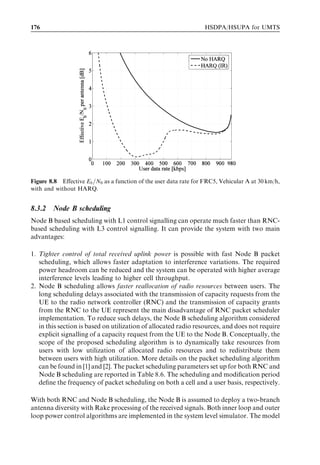
![168 HSDPA/HSUPA for UMTS
In this chapter, we will attempt to adhere closely to the basic assumptions agreed in the
Third Generation Partnership Project (3GPP). During the discussion of results, it will be
indicated which factors in the above play the most important roles.
The following performance metrics are used in this chapter:
. Average cell throughput – the average amount of data from all users in a cell that can
be received during a certain amount of time.
. 10% packet call throughput – representing the end user experience. It indicates the 10%
outage of user throughput (i.e., 90% of end users will experience a better packet call
throughput than this value).
. Eb =N0 – the required power per information bit over noise in order to receive a certain
bit rate with a certain block error probability. This has a direct impact on the load of
the system [16].
. Ec =N0 – the required power per chip bit over noise in order to receive a certain bit rate
with a certain block error probability.
Other less general measures will be introduced in addition to the presented results.
8.2 Single-user performance
The link performance of an enhanced uplink dedicated channel (E-DCH) link is studied
in this section. We use so-called ‘fixed reference channels’ (FRCs) in link level studies.
FRCs are a set of E-DCH channel configurations defined in 3GPP for performance
testing purposes. They are defined in [21] and shown in Table 8.1.
FRC1 to FRC3 use a 2-ms transmission time interval (TTI), whereas the other FRCs
are specified for a TTI of 10 ms. The maximum bit rate varies with the number of codes
with FRC3 providing a peak bit rate of more than 4 Mbps. The 3GPP performance
requirements using these FRCs are specified in [19]. The requirements specify a minimum
performance under certain conditions.
For each FRC, there exists one pair of suggested power ratios between the enhanced
dedicated physical data channel (E-DPDCH), the enhanced dedicated physical control
Table 8.1 Fixed reference channels (FRCs) defined for E-DCH.
FRC TTI Transport Codes Coding rate Maximum UE category
length block size bit rate
(ms) (bits) (kbps)
1 2 2 688 2*SF4 0.71 1353 2
2 2 5 376 2*SF2 0.71 2706 4
3 2 8 064 2*SF4 þ 2*SF2 0.71 4059 6
4 10 4 800 1*SF4 0.53 508 1
5 10 9 600 2*SF4 0.51 980 2 and 3
6 10 19 200 2*SF2 0.51 1960 4 and 5
7 10 640 1*SF16 0.29 69 1](https://image.slidesharecdn.com/wileyhsdpahsupaforumts-12712250730845-phpapp02/85/Hsdpa-Hsupa-For-Umts-192-320.jpg)
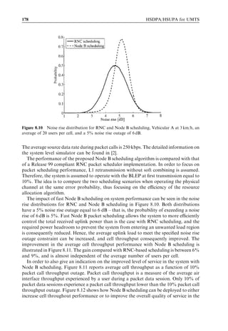
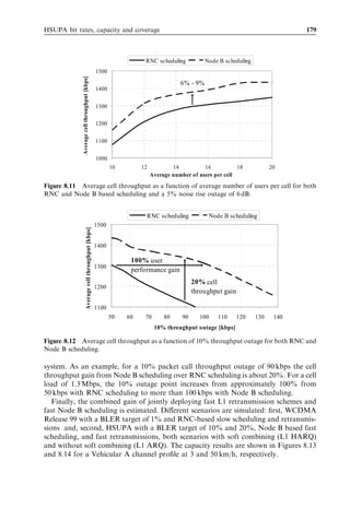
![HSUPA bit rates, capacity and coverage 171
Figure 8.2 E-DPCCH DTX detection performance for a 2-ms TTI.
7
6
Noise rise over thermal [dB]
5
4
3
2
1
0
-20 -15 -10 -5 0 5
Ec/N0 [dB]
Figure 8.3 Uplink noise rise caused by single user as a function of required Ec =N0 .
Figure 8.4 shows single-user uplink throughput on the radio link control (RLC) level
in kbps vs the received signal code power (RSCP) of the common pilot channel (CPICH)
in the UE. A lower RSCP means a larger path loss and, thus, a lower uplink throughput.
The throughput is assumed to be limited by the maximum UE power level – capacity
and packet scheduling aspects are not considered. The peak bit rate of 1.4 Mbps that is](https://image.slidesharecdn.com/wileyhsdpahsupaforumts-12712250730845-phpapp02/85/Hsdpa-Hsupa-For-Umts-195-320.jpg)
![172 HSDPA/HSUPA for UMTS
Table 8.4 Assumptions for user bit rate analysis.
Maximum UE bit rate Category 3 with maximum 1.45 Mbps
Maximum UE transmission power Class 3 with maximum 24 dBm
Base station noise level À105 dBm
CPICH power level 33 dBm
RLC overhead 5%
Slow fading standard deviation 8 dB
2000
HSUPA 1.45 Mbps
1800 WCDMA 384 kbps
1600
1400
RLC data rate [kbps]
1200
1000
800
600
400
200
0
-115 -110 -105 -100 -95 -90 -85 -80
RSCP [dBm]
Figure 8.4 Instantaneous single-user uplink throughput vs CPICH RSCP.
characteristic of a HSUPA Category 3 UE can be achieved with an RSCP of À92 dBm.
HSUPA provides a clearly higher data rate than a wideband code division multiple
access (WCDMA) 384-kbps UE when the RSCP level is higher than approximately
À100 dBm. HSUPA also provides some gain in throughput with lower RSCP levels due
to faster L1 HARQs.
Figure 8.5 shows the cumulative distribution of the uplink single-user data rate over
the area of a large macro-cell including shadow fading and soft handover. The cell size is
defined so that 64 kbps can be provided with a 95% coverage probability. An uplink rate
of 384 kbps can be offered with 70% probability and 1.4-Mbps HSDPA with approxi-
mately a 40% probability from the UE power point of view.
The average bit rate and the 95% bit rate from Figure 8.5 are illustrated in Table 8.5.
HSUPA can take benefit of the higher peak bit rate than that of WCDMA and can
provide a 2.7Â higher average bit rate than WCDMA. There is some gain from HSUPA
at the 95% probability point, but that gain is clearly less than the gain in terms of the
average data rate.](https://image.slidesharecdn.com/wileyhsdpahsupaforumts-12712250730845-phpapp02/85/Hsdpa-Hsupa-For-Umts-196-320.jpg)
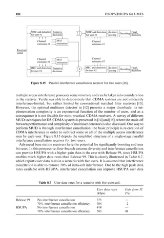
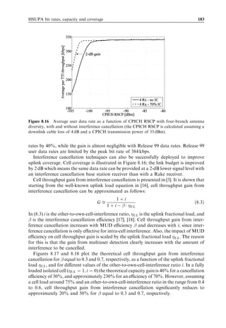
![HSUPA bit rates, capacity and coverage 175
Figure 8.7 Effective Eb =N0 vs BLEP at first transmission for FRC5, Vehicular A at 30 km/h, with
and without HARQ.
For a given received energy per bit-to-noise ratio, incremental redundancy provides a
lower frame erasure rate than is the case with no HARQ, thus leading to higher user
throughput. The gain from incremental redundancy (HARQ) clearly depends on the
system operation point: the higher the required Eb =N0 , the lower the target BLEP at first
transmission and the lower the gain from HARQ.
Following the definition of cell throughput in [16], uplink spectral efficiency is inversely
proportional to the effective Eb =N0 . The optimal operation point typically depends on
the propagation and mobility scenario, as well as on whether or not combining tech-
niques are used. The results reported in Figure 8.7 show how uplink spectral efficiency
can be improved by increasing the BLEP at first transmission, which leads to a lower
Eb =N0 requirement. This is possible since the low round trip delay with L1 retransmission
schemes allows fast recovery from transmission errors. For instance, spectral efficiency
gain from increasing the BLEP at first transmission from 1% to 10% is between 0.6 and
0.7 dB, corresponding to a cell throughput increase of approximately 15–20%.
Incremental redundancy can be successfully deployed to further increase uplink
spectral efficiency, although the gain from HARQ is really appreciable only for FER
values above 50%. In Figure 8.8, the effective Eb =N0 with incremental redundancy is
minimized at 300 kbps, which corresponds to an FER of approximately 70%, and to a
BLEP at first transmission higher than 90% in Figure 8.7. Assuming that with RLC
retransmissions the physical channel is operated at an error probability of 1%, the
maximum spectral efficiency gain from L1 HARQ is approximately 2 dB, corresponding
to a cell throughput increase of 60%. However, the price to pay is significantly increased
transmission delay, reduced user data rate, as well as more processing power at the base
station due to multiple retransmissions. Assuming a more realistic operation region for
the BLEP at first transmission between 20% and 30%, the cell throughput gain from L1
HARQ is approximately 15% to 20%.](https://image.slidesharecdn.com/wileyhsdpahsupaforumts-12712250730845-phpapp02/85/Hsdpa-Hsupa-For-Umts-199-320.jpg)
![176 HSDPA/HSUPA for UMTS
Figure 8.8 Effective Eb =N0 as a function of the user data rate for FRC5, Vehicular A at 30 km/h,
with and without HARQ.
8.3.2 Node B scheduling
Node B based scheduling with L1 control signalling can operate much faster than RNC-
based scheduling with L3 control signalling. It can provide the system with two main
advantages:
1. Tighter control of total received uplink power is possible with fast Node B packet
scheduling, which allows faster adaptation to interference variations. The required
power headroom can be reduced and the system can be operated with higher average
interference levels leading to higher cell throughput.
2. Node B scheduling allows faster reallocation of radio resources between users. The
long scheduling delays associated with the transmission of capacity requests from the
UE to the radio network controller (RNC) and the transmission of capacity grants
from the RNC to the UE represent the main disadvantage of RNC packet scheduler
implementation. To reduce such delays, the Node B scheduling algorithm considered
in this section is based on utilization of allocated radio resources, and does not require
explicit signalling of a capacity request from the UE to the Node B. Conceptually, the
scope of the proposed scheduling algorithm is to dynamically take resources from
users with low utilization of allocated radio resources and to redistribute them
between users with high utilization. More details on the packet scheduling algorithm
can be found in [1] and [2]. The packet scheduling parameters set up for both RNC and
Node B scheduling are reported in Table 8.6. The scheduling and modification period
define the frequency of packet scheduling on both a cell and a user basis, respectively.
With both RNC and Node B scheduling, the Node B is assumed to deploy a two-branch
antenna diversity with Rake processing of the received signals. Both inner loop and outer
loop power control algorithms are implemented in the system level simulator. The model](https://image.slidesharecdn.com/wileyhsdpahsupaforumts-12712250730845-phpapp02/85/Hsdpa-Hsupa-For-Umts-200-320.jpg)
![HSUPA bit rates, capacity and coverage 177
Table 8.6 Packet scheduling parameter setup for simulation of RNC and Node B scheduling.
Node B scheduling RNC scheduling
(ms)
Packet scheduling period 100 200 ms
User data rate modification period 100 600 ms
Allocation delay 40 100 ms
Inactivity timer
After having been inactive for this time period a UE 100 2s
is downgraded to the minimum allowed data rate
also includes soft and softer handover, with selection diversity performed at the RNC for
soft handover, and maximal ratio combining at the Node B for softer handover.
The model used to simulate packet data traffic is the modified gaming model described
in [5]. As illustrated in Figure 8.9, the state of a simulated user with respect to the
generation and transmission of data packets can be divided into three main phases:
1. In the first phase of the packet call, source data are generated in the user RLC buffer.
During this first phase, data are transmitted based on both buffer occupancy and the
data rate allocated by the packet scheduler.
2. During the second phase, the generation of source data in the user RLC buffer is
terminated. At the same time, the terminal continues transmitting the data it has
accumulated during the packet call period. This second phase is ended whenever all
the buffered data have been successfully transmitted.
3. Finally, during the third phase no data are generated in the user RLC buffer. This
phase is considered ‘reading time’. Since the buffer is empty when the third phase
starts, during reading time no data are transmitted.
End of packet Start of new
call packet call
Packet call: packets are Reading time
generated into the RLC buffer
Packet inter-arrival
time Transmission of data packets RLC buffer is empty: the
accumulated during the active reading time is started
period. No new packets are
generated
Figure 8.9 Source traffic model and its closed loop feature.](https://image.slidesharecdn.com/wileyhsdpahsupaforumts-12712250730845-phpapp02/85/Hsdpa-Hsupa-For-Umts-201-320.jpg)
![178 HSDPA/HSUPA for UMTS
Figure 8.10 Noise rise distribution for RNC and Node B scheduling, Vehicular A at 3 km/h, an
average of 20 users per cell, and a 5% noise rise outage of 6 dB.
The average source data rate during packet calls is 250 kbps. The detailed information on
the system level simulator can be found in [2].
The performance of the proposed Node B scheduling algorithm is compared with that
of a Release 99 compliant RNC packet scheduler implementation. In order to focus on
packet scheduling performance, L1 retransmission without soft combining is assumed.
Therefore, the system is assumed to operate with the BLEP at first transmission equal to
10%. The idea is to compare the two scheduling scenarios when operating the physical
channel at the same error probability, thus focusing on the efficiency of the resource
allocation algorithm.
The impact of fast Node B scheduling on system performance can be seen in the noise
rise distributions for RNC and Node B scheduling in Figure 8.10. Both distributions
have a 5% noise rise outage equal to 6 dB – that is, the probability of exceeding a noise
rise of 6 dB is 5%. Fast Node B packet scheduling allows the system to more efficiently
control the total received uplink power than is the case with RNC scheduling, and the
required power headroom to prevent the system from entering an unwanted load region
is consequently reduced. Hence, the average uplink load to meet the specified noise rise
outage constraint can be increased, and cell throughput consequently improved. The
improvement in the average cell throughput performance with Node B scheduling is
illustrated in Figure 8.11. The gain compared with RNC-based scheduling is between 6%
and 9%, and is almost independent of the average number of users per cell.
In order to also give an indication on the improved level of service in the system with
Node B scheduling, Figure 8.11 reports average cell throughput as a function of 10%
packet call throughput outage. Packet call throughput is a measure of the average air
interface throughput experienced by a user during a packet data session. Only 10% of
packet data sessions experience a packet call throughput lower than the 10% packet call
throughput outage. Figure 8.12 shows how Node B scheduling can be deployed to either
increase cell throughout performance or to improve the overall quality of service in the](https://image.slidesharecdn.com/wileyhsdpahsupaforumts-12712250730845-phpapp02/85/Hsdpa-Hsupa-For-Umts-202-320.jpg)
![HSUPA bit rates, capacity and coverage 179
RNC scheduling Node B scheduling
1500
Average cell throughput [kbps] 6% - 9%
1400
1300
1200
1100
1000
10 12 14 16 18 20
Average number of users per cell
Figure 8.11 Average cell throughput as a function of average number of users per cell for both
RNC and Node B based scheduling and a 5% noise rise outage of 6 dB.
RNC scheduling Node B scheduling
1500
Average cell throughput [kbps]
1400
100% user
1300
performance gain
20% cell
1200
throughput gain
1100
50 60 70 80 90 100 110 120 130 140
10% throughput outage [kbps]
Figure 8.12 Average cell throughput as a function of 10% throughput outage for both RNC and
Node B scheduling.
system. As an example, for a 10% packet call throughput outage of 90 kbps the cell
throughput gain from Node B scheduling over RNC scheduling is about 20%. For a cell
load of 1.3 Mbps, the 10% outage point increases from approximately 100% from
50 kbps with RNC scheduling to more than 100 kbps with Node B scheduling.
Finally, the combined gain of jointly deploying fast L1 retransmission schemes and
fast Node B scheduling is estimated. Different scenarios are simulated: first, WCDMA
Release 99 with a BLER target of 1% and RNC-based slow scheduling and retransmis-
sions and, second, HSUPA with a BLER target of 10% and 20%, Node B based fast
scheduling, and fast retransmissions, both scenarios with soft combining (L1 HARQ)
and without soft combining (L1 ARQ). The capacity results are shown in Figures 8.13
and 8.14 for a Vehicular A channel profile at 3 and 50 km/h, respectively.](https://image.slidesharecdn.com/wileyhsdpahsupaforumts-12712250730845-phpapp02/85/Hsdpa-Hsupa-For-Umts-203-320.jpg)
![180 HSDPA/HSUPA for UMTS
L2 ARQ L1 ARQ L1 HARQ
Average cell throughput [kbps] 1600
26% 27%
21% 25%
1400
1200
1000
800
600
400
200
0
RNC - 1% Node B - 10% Node B - 20%
Figure 8.13 Average cell throughput with Vehicular A at 3 km/h, 5% noise rise outage of 6 dB,
and 10% throughput outage of 64 kbps.
L2 ARQ HARQ type-I HARQ type-II
1600
Average cell throughput [kbps]
1400 59%
53%
50% 52%
1200
1000
800
600
400
200
0
RNC - 1% Node B - 10% Node B - 20%
Figure 8.14 Average cell throughput with Vehicular A at 50 km/h, 5% noise rise outage of 6 dB,
and 10% throughput outage of 64 kbps.
Under the assumptions considered, the cell throughput gain of HSUPA compared
with WCDMA Release 99 is 25% to 60%, depending on the mobility scenario. The
reason for a higher cell throughput gain with a UE speed of 50 km/h can be explained
by the higher spectral efficiency gain when increasing the BLEP target at first trans-
mission from 1% to 10%. The reason is that a low BLEP is more difficult to achieve
at high mobile speed since power control accuracy is not as good as at low mobile
speed.
Most of the gain from L1 retransmission schemes is obtained from operating the
physical channel at a higher error probability, rather than from deploying soft combining
techniques. Node B based scheduling provides a cell throughput increase of approxi-
mately 15% to 20% on top of the gain from L1 HARQ.](https://image.slidesharecdn.com/wileyhsdpahsupaforumts-12712250730845-phpapp02/85/Hsdpa-Hsupa-For-Umts-204-320.jpg)
![HSUPA bit rates, capacity and coverage 181
8.4 HSUPA performance enhancements
Uplink spectral efficiency and data rates can be improved with antenna and baseband
solutions. This section briefly introduces antenna diversity, beamforming, interference
rejection combining, and multiuser detection (MUD).
Multibranch antenna diversity and beamforming – antenna arrays can be operated in two
distinct modes: (i) diversity mode or (ii) beamforming mode. Diversity techniques rely on
the statistical independence between antenna elements to reduce the likelihood of deep
fades, and are additionally able to provide an average signal-to-interference-plus-noise
ratio (SINR) gain by coherently combining the signals received at each antenna element
[9]. Beamforming techniques direct narrow beams towards each user in such a way that
multiple access interference is reduced by means of spatial filtering and potential
suppression of interfering signals [11]. The basic choice is whether to maximize diversity
or antenna gain. In [13] performance evaluation of different antenna array approaches
for the WCDMA uplink is presented. It is shown how diversity and beamforming
concepts perform similarly with a small number of antennas per sector, while the
conventional beamforming approach starts to overcome diversity techniques with a
large number of antennas and low azimuth spread. However, diversity techniques are
shown to perform better in low-mobility environments since longer averaging periods
can be applied for better channel estimates. Also, in [15] it is shown that for channel
environments with a large angular spread, space diversity schemes with interference
cancellation represent an attractive solution compared with beamforming in terms of
complexity and robustness, against calibration errors of the antenna array.
The choice of antenna solution must consider both uplink and downlink requirements.
See the downlink HSDPA performance discussion in Chapter 7. Beamforming mode
looks attractive for enhancing downlink performance.
Interference rejection combining – traditional antenna diversity combining uses maximal
ratio combining (MRC) where interference is assumed to be spatially white. Interference
rejection combining (IRC) exploits the spatial properties of interference [28]. MRC aims
to maximize the received signal power while IRC aims to maximize the received signal-to-
interference ratio. IRC can improve performance substantially in the case of dominant
interferers. Since HSUPA enables high peak data rates, thus possibly leading to
interference scenarios characterized by dominant interferers, IRC has the potential to
provide significant capacity and coverage gains. In case of low data rate users in
WCDMA, there are no dominant interferers, and the IRC receiver cannot provide
any gains. Implementation of an IRC receiver is relatively simple compared with employ-
ing the MUD algorithm. IRC algorithms are used in Global System for Mobile
Communications (GSM) base station receivers to improve performance since dominant
interferers are typical in the GSM system.
Multiuser detection – although multiple access interference (MAI) is often approximated
as additive white Gaussian noise (AWGN) [11], in reality it consists of the distinct
received signals of code division multiple access (CDMA) users. As a consequence,](https://image.slidesharecdn.com/wileyhsdpahsupaforumts-12712250730845-phpapp02/85/Hsdpa-Hsupa-For-Umts-205-320.jpg)
![182 HSDPA/HSUPA for UMTS
MRC and detection Tentative + MRC and detection de-inter- Final
for user #1 S Decoding
decisions - for user #1 leaving decisions
Channel MAI Channel
estimates #1 estimation estimates #1
Received
signal
Channel MAI Channel
estimates #2 estimation estimates #2
- MRC and detection de-inter- Final
MRC and detection Tentative S Decoding
for user #2 decisions + for user #2 leaving decisions
Figure 8.15 Parallel interference cancellation receiver for two users [16].
multiple access interference possesses some structure and can be taken into consideration
in the receiver. Verdu was able to demonstrate that CDMA systems are not inherently
´
interference-limited, but rather limited by conventional matched filter receivers [13].
However, the optimal multiuser detector in [12] presents a major drawback: its im-
plementation complexity is an exponential function of the number of users, and as a
consequence it is not feasible for most practical CDMA receivers. A survey of different
MUD techniques for DS-CDMA systems is presented in [14] and [15], where the trade-off
between performance and complexity of multiuser detectors is also discussed. One way to
perform MUD is through interference cancellation: the basic principle is re-creation of
CDMA interference in order to subtract some or all of the multiple access interference
seen by each user. Figure 8.15 depicts the simplified structure of a single-stage parallel
interference cancellation receiver for two users.
Advanced base station receivers have the potential for significantly boosting end user
bit rates. In this perspective, four-branch antenna diversity and interference cancellation
can provide HSUPA with a higher gain than is the case with Release 99, since HSUPA
enables much higher data rates than Release 99. This is clearly illustrated in Table 8.7,
which reports user data rates in a scenario with five users. It is assumed that interference
cancellation is able to remove 70% of intra-cell interference. Due to the high peak data
rates available with HSUPA, interference cancellation can improve HSUPA user data
Table 8.7 User data rates for a scenario with five users/cell.
User data rates Gain from IC
(kbps) (%)
Release 99 No interference cancellation 375 —
70% interference cancellation efficiency 384 2
HSUPA No interference cancellation 414 —
70% interference cancellation efficiency 583 41](https://image.slidesharecdn.com/wileyhsdpahsupaforumts-12712250730845-phpapp02/85/Hsdpa-Hsupa-For-Umts-206-320.jpg)
![HSUPA bit rates, capacity and coverage 183
Figure 8.16 Average user data rate as a function of CPICH RSCP with four-branch antenna
diversity, with and without interference cancellation (the CPICH RSCP is calculated assuming a
downlink cable loss of 4 dB and a CPICH transmission power of 33 dBm).
rates by 40%, while the gain is almost negligible with Release 99 data rates. Release 99
user data rates are limited by the peak bit rate of 384 kbps.
Interference cancellation techniques can also be successfully deployed to improve
uplink coverage. Cell coverage is illustrated in Figure 8.16; the link budget is improved
by 2 dB which means the same data rate can be provided at a 2-dB lower signal level with
an interference cancellation base station receiver than with a Rake receiver.
Cell throughput gain from interference cancellation is presented in [3]. It is shown that
starting from the well-known uplink load equation in [16], cell throughput gain from
interference cancellation can be approximated as follows:
1þi
Gffi ð8:3Þ
1 þ i À](https://image.slidesharecdn.com/wileyhsdpahsupaforumts-12712250730845-phpapp02/85/Hsdpa-Hsupa-For-Umts-207-320.jpg)
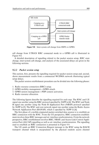
![is the interference cancellation efficiency [17], [18]. Cell throughput gain from inter-
ference cancellation increases with MUD efficiency](https://image.slidesharecdn.com/wileyhsdpahsupaforumts-12712250730845-phpapp02/85/Hsdpa-Hsupa-For-Umts-209-320.jpg)
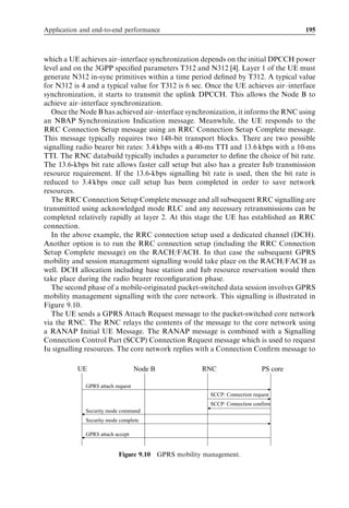
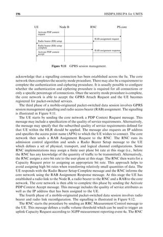
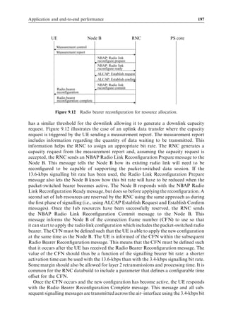
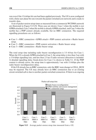
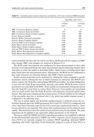
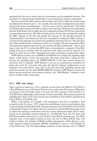
![HSUPA bit rates, capacity and coverage 185
Vehicular A 3 km/h - 5% NR outage = 6 dB
10% PCT outage = 64 kbps 10% PCT outage = 128 kbps
5
RNC PS 295%
Average cell throughput [Mbps]
Node B PS
4
208%
159%
3
2
29%
1
0
2 Rx - no IC 2 Rx - no IC 4 Rx - no IC 4 Rx - 30% IC 4 Rx - 70% IC
Figure 8.19 Average cell throughput for different antenna diversity and IC scenarios with Node B
PS and L1 HARQ, and compared with the performance of a reference Release 99 scenario (RNC
PS and L2 ARQ).
tion which enables efficient mobile power amplifier operation and facilitates good
coverage for high data rates. From the coverage point of view, high HSUPA bit
rates above 1 Mbps are even available in a large macro-cell at a 50% probability.
HSUPA uses advanced techniques to also improve cell capacity and spectral efficiency
in loaded cells. The techniques include fast L1 retransmissions with HARQ and fast
Node B based scheduling. Fast retransmissions allow a higher error rate in HSUPA than
in the Release 99 DCH while still maintaining the same end-to-end delay. If the block
error rate is increased from 1% to 10%, cell capacity gain is 15–20%, and with higher
block error rate levels even beyond 50%. Fast Node B scheduling allows using higher
average interference levels in HSUPA than in the Release 99 DCH since fast scheduling
makes signal-to-interference distribution narrow and reduces the interference outage
probability. The capacity gain from fast scheduling is 10–20% depending on the required
outage probability. In total, the expected capacity gain from HSUPA is 25–60%.
HSUPA cell capacity can be further improved by using base station antenna beam-
forming, four-branch reception, interference rejection combining, and interference
cancellation. All solutions are supported by the current 3GPP HSUPA standard.
These techniques can reduce the amount of interference and, thus, provide higher
data rates and higher cell capacity.
8.6 Bibliography
[1] C. Rosa, J. Outes, K. Dimou, T. B. Sørensen, J. Wigard, F. Frederiksen, and P. E.
Mogensen (2004), Performance of fast Node B scheduling and L1 HARQ schemes in
WCDMA uplink packet access, IEEE Proceedings of the 59th Vehicular Technology Con-
ference, May.](https://image.slidesharecdn.com/wileyhsdpahsupaforumts-12712250730845-phpapp02/85/Hsdpa-Hsupa-For-Umts-216-320.jpg)
![186 HSDPA/HSUPA for UMTS
[2] C. Rosa (2004), Enhanced uplink packet access in WCDMA, Ph.D. thesis, Aalborg Uni-
versity (Denmark), December.
[3] C. Rosa, T. B. Sørensen, J. Wigard, and P. E. Mogensen (2005), Interference cancellation
and 4-branch antenna diversity for WCDMA uplink packet access, IEEE Proceedings of the
61st Vehicular Technology Conference, May/June.
[4] 3GPP, Technical Specification Group RAN, Feasibility Study for Enhanced Uplink for
UTRA FDD, 3GPP TR 25.896 version 6.0.0, Release 6, March 2004, available at
www.3gpp.org
[5] T. Hytonen (2001), Optimal Wrap-Around Network Simulation, Helsinki University of
¨
Technology Report, A432.
[6] R. H. Clarke (1968), A statistical theory of mobile-radio reception, Bell Systems Technical
Journal, 47, 957–1000.
[7] W. C. Jakes (1974), Microwave Mobile Communications, IEEE Press, Los Alametos, CA.
[8] J. Ramiro-Moreno (2003), System level performance analysis of advanced antenna concepts
in WCDMA, Ph.D. thesis, Aalborg University (Denmark), July.
[9] J. Ylitalo and E. Tiirola (2000), Performance evaluation of different antenna array
approaches for 3G CDMA uplink, IEEE Proceedings of the 51st Vehicular Technology
Conference, May, Vol. 2, pp. 883–887.
[10] D. Dahlhaus and Zhenlan Cheng (2000), Smart antenna concepts with interference cancella-
tion for joint demodulation in the WCDMA UTRA uplink, IEEE Proceedings of the 6th
International Symposium on Spread Spectrum Techniques and Applications, September, Vol. 1,
pp. 244–248.
[11] J. G. Prakis (1995), Digital Communications, McGraw-Hill, London.
[12] S. Verdu (1986), Minimum probability of error for asynchronous Gaussian multiple-access
´
channels, IEEE Transactions on Information Theory, 32(1), 85–96, January.
[13] S. Verdu (1998), Multi-user Detection, Cambridge University Press, New York.
´
[14] A. Duel-Hallen, J. Holtzman, and Z. Zvonar (1995), Multiuser detection for CDMA
systems, IEEE Personal Communications, 2(2), 46–58, April.
[15] S. Moshavi (1996), Multi-user detection for DS-CDMA communications, IEEE Commun-
ications Magazine, 34(10), 124–136, October.
[16] H. Holma and A. Toskala (2004), WCDMA for UMTS: Radio Access for Third Generation
Mobile Communications (3rd edn), John Wiley Sons, Chichester, UK.
[17] B. Hagerman, F. Gunnarsson, H. Murai, M. Tadenuma, and J. Karlsson (2004), WCDMA
uplink interference cancellation performance: Field measurements and system simulations,
Nordic Radio Symposium, Session 10 – WCDMA Enhancements, August.
[18] S. Hamalainen, H. Holma, and A. Toskala (1996), Capacity evaluation of a cellular CDMA
¨ ¨ ¨
uplink with multiuser detection, IEEE Proceedings of the 4th International Symposium on
Spread Spectrum Techniques and Applications, September, Vol. 1, pp. 339–343.
[19] 3GPP, Technical Specification Group RAN, Base Station Radio Transmission and Recep-
tion, 3GPP TR 25.104 version 6.9.0, Release 6, June 2005, available at www.3gpp.org
[20] 3GPP, Technical Specification Group RAN, Physical Layer – Measurements (FDD), 3GPP
TS 25.215 version 6.3.0, Release 6, June 2005, available at www.3gpp.org
[21] 3GPP, R4-050315, EUL UL Simulation Assumptions, May 2005, available at www.3gpp.org
[22] D. Astely and A. Artamo (2001), Uplink spatio-temporal interference rejection combining
for WCDMA, IEEE Third Workshop on Signal Processing Advances in Wireless Commun-
ications (SPAWC ’01), 20–23 March, pp. 326–329.](https://image.slidesharecdn.com/wileyhsdpahsupaforumts-12712250730845-phpapp02/85/Hsdpa-Hsupa-For-Umts-217-320.jpg)
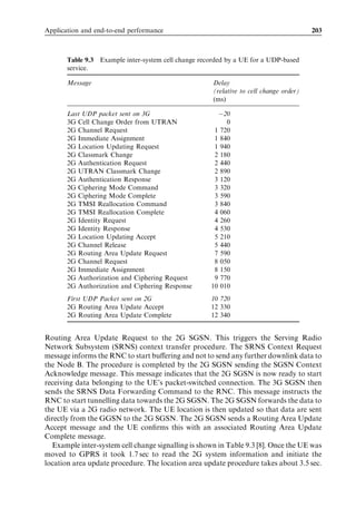
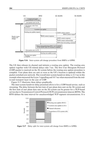
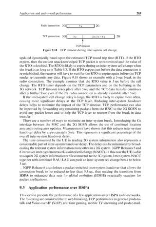
![190 HSDPA/HSUPA for UMTS
(a)
(b)
(c)
Figure 9.4 Use cases for broadband data access: (a) fixed broadband access (wireless DSL);
(b) portable broadband access (similar to hot spots); and (c) mobile broadband access (cellular
data access).
networks can provide data rates that are similar to fixed line broadband access. The
use cases are illustrated in Figure 9.4.
9.2 Always-on connectivity
9.2.1 Packet core and radio connectivity
Always-on connectivity is required to provide push services, like push e-mail and push-
to-talk, from the server to the terminal. The always-on capability also improves the end
user performance of interactive services by avoiding setup delays. It is not practical to
maintain the physical radio connection all of the time, but the network must be able to
maintain a logical connection without physical resource allocation.
An always-on application can preserve its transport layer connections if it can keep the
same Internet Protocol (IP) address despite its mobility. The IP address in a Universal
Mobile Telecommunications System (UMTS) network is allocated as part of the Packet
Data Protocol (PDP) context during GPRS session management [3]. Mobility manage-
ment must be maintained in the Serving GPRS Support Node (SGSN) which knows the
location of the mobile with routing area accuracy. Mobility information can also be
maintained in the radio network controller (RNC) which may know the location of the
mobile with cell or with UTRAN registration area (URA) accuracy. The mobility
management connection between the user equipment (UE) and the SGSN is created
by means of General Packet Radio Service (GPRS) attach signalling [3]. The radio
resource management connection to the RNC is obtained by radio resource control
(RRC) connection setup signalling. The different levels of connectivity are illustrated in
Figure 9.5.](https://image.slidesharecdn.com/wileyhsdpahsupaforumts-12712250730845-phpapp02/85/Hsdpa-Hsupa-For-Umts-221-320.jpg)
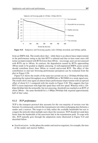
![192 HSDPA/HSUPA for UMTS
RRC connected Activity Buffer threshold
detection 128-1024 B
URA_PCH Cell_PCH Cell_FACH Cell_DCH
GPRS attached
Mobility = frequent Inactivity Inactivity/low
cell changes timer 2-10 s activity timer 2-10 s
RRC idle
Inactivity timer Activity
or RNC load detection
Idle
Figure 9.6 RRC states for packet-switched services.
300
200-300 mA
250
Power consumption [mA]
200
150
100-150 mA
100
50
5 mA
0
URA_PCH / Cell_FACH Cell_DCH
Cell_PCH / Idle
Figure 9.7 Indicative terminal power consumption in different RRC states.
must be on in order to decode any FACH messages. Therefore, power consumption in
Cell_FACH state is still relatively higher than in paging channel (PCH) states where the
UE only receives paging messages and can utilize sleep mode. The UE should be moved
relatively quickly to PCH state when the data transmission is over in order to minimize
UE power consumption.
RRC state changes are controlled by the operator using RNC parameters. A UE
cannot decide to make state changes itself.
When a UE goes beyond the wideband code division multiple access (WCDMA)/
HSPA coverage area during packet data transmission, the RNC will command the UE to
make an inter-system cell change to a GPRS cell. The IP address is preserved despite the
cell change, and any active packet applications remain connected since the same Gateway
GPRS Support Node (GGSN) is used both for HSPA and for GPRS. The inter-system](https://image.slidesharecdn.com/wileyhsdpahsupaforumts-12712250730845-phpapp02/85/Hsdpa-Hsupa-For-Umts-223-320.jpg)
![Application and end-to-end performance 193
Idle mode
Camping on aa
Camping on UTRAN RRC
UTRAN RRC
UTRAN cell
UTRAN cell connected mode
connected mode
Inter-system cell change
Camping on aaGPRS
Camping on GPRS GPRS Packet
GPRS Packet
cell
cell transfer mode
transfer mode
Figure 9.8 Inter-system cell change from HSPA to GPRS.
cell change from UTRAN RRC connected mode to a GPRS cell is illustrated in
Figure 9.8.
A detailed description of signalling related to the packet session setup, RRC state
change, inter-system cell change, and analysis of the associated delays are given in the
following sections.
9.2.2 Packet session setup
This section, first, presents the signalling required for packet session setup and, second,
shows measurement results from a commercial WCDMA network illustrating typical
setup delays.
The packet session establishment procedure can be divided into the following phases:
1. Radio resource connection (RRC) setup.
2. GPRS mobility management ¼ GPRS attach.
3. GPRS session management ¼ PDP context activation.
4. Radio resource allocation.
The following figures describe the signalling required for each step. The RNC and UE
signal one another using the RRC protocol specified by 3GPP in [4]. The RNC and Node
B signal one another using the Node B Application Part (NBAP) protocol specified
by 3GPP in [5]. The RNC and core network signal one another using the Radio Access
Network Application Part (RANAP), which is specified by 3GPP in [6].
The first phase of a mobile-originated packet-switched data session is to establish an
RRC connection with the RNC. From the UE perspective, RRC connection establish-
ment involves three RRC messages and air–interface synchronization. From the network
perspective, RRC establishment involves RRC, NBAP, and Access Link Control Appli-
cation Part (ALCAP) signalling as well as air–interface synchronization. The signalling
used to establish an RRC connection is presented in Figure 9.9.
The UE sends an RRC Connection Request message to the RNC using the RACH
transport channel which is encapsulated by the physical random access channel](https://image.slidesharecdn.com/wileyhsdpahsupaforumts-12712250730845-phpapp02/85/Hsdpa-Hsupa-For-Umts-224-320.jpg)
![194 HSDPA/HSUPA for UMTS
UE Node B RNC PS core
RRC connection request
(RACH)
NBAP: Radio link setup
request
NBAP: Radio link setup
response
ALCAP: Establish request
ALCAP: Establish confirm
RRC connection setup
(FACH)
L1 synchronization NBAP: Synchronization
indication
RRC connection setup
complete (DCH)
Figure 9.9 Radio resource control (RRC) connection setup.
(PRACH). Transmission on the PRACH physical channel must be preceded by the
transmission of uplink PRACH power control pre-ambles and their subsequent
acknowledgement by the Node B. Once the PRACH power control pre-ambles
have been acknowledged, the RRC Connection Request message can be sent. The
RRC Connection Request message is relatively small and requires only a single transport
block which is typically transmitted using a 20-ms transmission time interval (TTI) and
transparent mode radio link control (RLC). The RRC Connection Request message can
be retransmitted if necessary based upon 3GPP parameters N300 and T300 [5]. These
parameters are broadcast to the UE in system information block 1.
Once the RNC has received the RRC Connection Request message it uses NBAP
signalling to request a radio link at the relevant Node B. The Node B starts to transmit a
dedicated physical control channel (DPCCH) for the new radio link. The transmit power
is based upon a downlink open loop power control calculation. The RNC then reserves
an associated set of Iub transmission resources using the ALCAP Establish Request and
Establish Confirm messages. The RNC responds to the UE’s RRC Connection Request
message using an RRC Connection Setup message. This message is transmitted using the
FACH transport channel. The RRC Connection Setup message is relatively large and
typically requires seven transport blocks. These transport blocks have a size of 168 bits
and are transmitted using a 10-ms TTI and unacknowledged mode RLC. The transport
block set size is typically defined such that a maximum of two transport blocks can be
sent per 10-ms TTI. If the UE is in an area of poor downlink coverage, then it is possible
that it does not receive one or more of the RRC Connection Setup message transport
blocks. In this case the RNC is required to retransmit the complete set of transport blocks
from layer 3. The parameters defining retransmission of the RRC Connection Setup
message are not specified by 3GPP. The RNC databuild may include implementation-
dependent parameters defining the period between retransmissions and the maximum
allowed number of retransmissions.
Once the UE has received the RRC Connection Setup message, it attempts to achieve
air–interface synchronization using the DPCCH transmitted by the Node B. The rate at](https://image.slidesharecdn.com/wileyhsdpahsupaforumts-12712250730845-phpapp02/85/Hsdpa-Hsupa-For-Umts-225-320.jpg)
![Application and end-to-end performance 195
which a UE achieves air–interface synchronization depends on the initial DPCCH power
level and on the 3GPP specified parameters T312 and N312 [4]. Layer 1 of the UE must
generate N312 in-sync primitives within a time period defined by T312. A typical value
for N312 is 4 and a typical value for T312 is 6 sec. Once the UE achieves air–interface
synchronization, it starts to transmit the uplink DPCCH. This allows the Node B to
achieve air–interface synchronization.
Once the Node B has achieved air–interface synchronization, it informs the RNC using
an NBAP Synchronization Indication message. Meanwhile, the UE responds to the
RRC Connection Setup message using an RRC Connection Setup Complete message.
This message typically requires two 148-bit transport blocks. There are two possible
signalling radio bearer bit rates: 3.4 kbps with a 40-ms TTI and 13.6 kbps with a 10-ms
TTI. The RNC databuild typically includes a parameter to define the choice of bit rate.
The 13.6-kbps bit rate allows faster call setup but also has a greater Iub transmission
resource requirement. If the 13.6-kbps signalling bit rate is used, then the bit rate is
reduced to 3.4 kbps once call setup has been completed in order to save network
resources.
The RRC Connection Setup Complete message and all subsequent RRC signalling are
transmitted using acknowledged mode RLC and any necessary retransmissions can be
completed relatively rapidly at layer 2. At this stage the UE has established an RRC
connection.
In the above example, the RRC connection setup used a dedicated channel (DCH).
Another option is to run the RRC connection setup (including the RRC Connection
Setup Complete message) on the RACH/FACH. In that case the subsequent GPRS
mobility and session management signalling would take place on the RACH/FACH as
well. DCH allocation including base station and Iub resource reservation would then
take place during the radio bearer reconfiguration phase.
The second phase of a mobile-originated packet-switched data session involves GPRS
mobility management signalling with the core network. This signalling is illustrated in
Figure 9.10.
The UE sends a GPRS Attach Request message to the packet-switched core network
via the RNC. The RNC relays the contents of the message to the core network using
a RANAP Initial UE Message. The RANAP message is combined with a Signalling
Connection Control Part (SCCP) Connection Request message which is used to request
Iu signalling resources. The core network replies with a Connection Confirm message to
UE Node B RNC PS core
GPRS attach request
SCCP: Connection request
SCCP: Connection confirm
Security mode command
Security mode complete
GPRS attach accept
Figure 9.10 GPRS mobility management.](https://image.slidesharecdn.com/wileyhsdpahsupaforumts-12712250730845-phpapp02/85/Hsdpa-Hsupa-For-Umts-226-320.jpg)
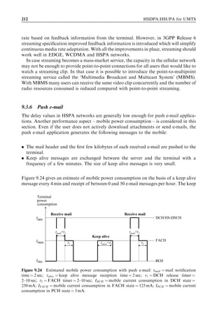
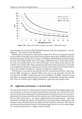
![198 HSDPA/HSUPA for UMTS
rate even if the 13.6-kbps bit rate had been applied previously. The UE is now configured
with a finite user plane bit rate towards the packet-switched core network and is ready to
transfer data.
A set of packet session setup times as measured from a commercial WCDMA network
are illustrated in Figure 9.13 [7]. Three case are shown: Case 1 when the mobile is not
GPRS-attached, Case 2 when the mobile is already GPRS-attached, and Case 3 when the
mobile has a PDP context already available, but no RRC connection. The required
signalling procedures are as follows:
. Case 1 ¼ RRC connection þ GPRS attach þ PDP context activation þ Radio bearer
setup.
. Case 2 ¼ RRC connection þ PDP context activation þ Radio bearer setup.
. Case 3 ¼ RRC connection þ Radio bearer setup.
The total setup time including radio bearer reconfiguration is 3.5–4.0 sec for Case 1.
When the UE is already GPRS-attached in Case 2, the setup delay is less than 2 sec with
a 13.6-kbps signalling rate, and less than 2.5 sec if radio resource allocation is included.
A detailed signalling delay break-down for Case 2 is shown in Table 9.1. If the PDP
context is already active, the setup time is approximately 1 sec with 13.6 kbps plus the
radio bearer reconfiguration delay.
If the UE already has an RRC connection, only the RRC state change to CELL_DCH
may be required. The UE may already have an RRC connection due to an existing
circuit-switched call or due to another packet-switched connection. If there is an ongoing
Packet call setup time
Radio bearer reconfiguration
4.5 GPRS mobility and session management
RRC connection setup
4.0
3.5
3.0
Seconds
2.5
2.0
1.5
1.0
0.5
0.0
Case 1 - Case 1 - Case 2 - Case 2 - Case 3 - Case 3 -
SRB13.6 SRB3.4 SRB13.6 SRB3.4 SRB 13.6 SRB3.4
kbps kbps kbps kbps kbps kbps
Figure 9.13 Average packet session setup time measured from a UE.](https://image.slidesharecdn.com/wileyhsdpahsupaforumts-12712250730845-phpapp02/85/Hsdpa-Hsupa-For-Umts-229-320.jpg)
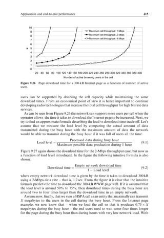
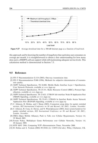
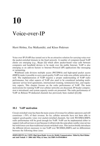
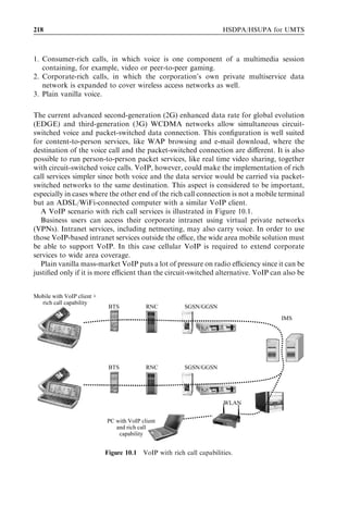
![Application and end-to-end performance 203
Table 9.3 Example inter-system cell change recorded by a UE for a UDP-based
service.
Message Delay
(relative to cell change order)
(ms)
Last UDP packet sent on 3G À20
3G Cell Change Order from UTRAN 0
2G Channel Request 1 720
2G Immediate Assignment 1 840
2G Location Updating Request 1 940
2G Classmark Change 2 180
2G Authentication Request 2 440
2G UTRAN Classmark Change 2 890
2G Authentication Response 3 120
2G Ciphering Mode Command 3 320
2G Ciphering Mode Complete 3 590
2G TMSI Reallocation Command 3 840
2G TMSI Reallocation Complete 4 060
2G Identity Request 4 260
2G Identity Response 4 530
2G Location Updating Accept 5 210
2G Channel Release 5 440
2G Routing Area Update Request 7 590
2G Channel Request 8 050
2G Immediate Assignment 8 150
2G Authorization and Ciphering Request 9 770
2G Authorization and Ciphering Response 10 010
First UDP Packet sent on 2G 10 720
2G Routing Area Update Accept 12 330
2G Routing Area Update Complete 12 340
Routing Area Update Request to the 2G SGSN. This triggers the Serving Radio
Network Subsystem (SRNS) context transfer procedure. The SRNS Context Request
message informs the RNC to start buffering and not to send any further downlink data to
the Node B. The procedure is completed by the 2G SGSN sending the SGSN Context
Acknowledge message. This message indicates that the 2G SGSN is now ready to start
receiving data belonging to the UE’s packet-switched connection. The 3G SGSN then
sends the SRNS Data Forwarding Command to the RNC. This message instructs the
RNC to start tunnelling data towards the 2G SGSN. The 2G SGSN forwards the data to
the UE via a 2G radio network. The UE location is then updated so that data are sent
directly from the GGSN to the 2G SGSN. The 2G SGSN sends a Routing Area Update
Accept message and the UE confirms this with an associated Routing Area Update
Complete message.
Example inter-system cell change signalling is shown in Table 9.3 [8]. Once the UE was
moved to GPRS it took 1.7 sec to read the 2G system information and initiate the
location area update procedure. The location area update procedure takes about 3.5 sec.](https://image.slidesharecdn.com/wileyhsdpahsupaforumts-12712250730845-phpapp02/85/Hsdpa-Hsupa-For-Umts-234-320.jpg)
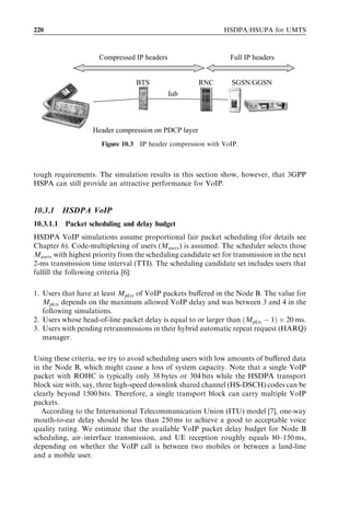
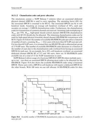
![206 HSDPA/HSUPA for UMTS
9.3.1 Web browsing
End users are increasingly accustomed to broadband web browsing performance
through fixed Internet connections. In comparison, the browsing performance over early
deployments of cellular systems supporting packet-switched services has suffered from
limited throughput and rather significant latencies. Due to the interactive nature of web
browsing, latency plays a particularly important role in determining perceived end user
performance. This is particularly true for user-to-network interface link speeds above a
few hundred kilobits per second, above which the effective end-to-end throughput seen
by the end user will be limited by other network links along the path. In comparison, the
effect of link RTT is cumulative over an end-to-end path. Thus, it is clearly the case that it
is link RTT, rather than link speed, that becomes a performance limiting factor.
The role of RTT on perceived link performance can be verified using the network setup
illustrated in Figure 9.19, where a network emulator is used to induce extrinsic delay on
the end-to-end communication link. This setup can be used as a platform for carrying out
subjective degradation category rating tests as defined in [2]. These tests are used for
judgements of pairs of links, where one of the links does not bear any extrinsic delay and
the other has been degraded by inducing some extrinsic delay. The links are compared
and the degradation of the manipulated link is rated on a scale from 1 to 5, where 1
corresponds to very annoying and 5 corresponds to unnoticeable degradation.
Figure 9.20 shows the results obtained from a degradation category rating test carried
out over a 1-Mbps/384-kbps link, emulating the typical throughput that can be expected
http://w w w .w iley.com
Network emulator
Laptop with (bit rate limiter and Public Public server
browser delay generator) Internet
Figure 9.19 Measurement setup for subjective web browsing measurements.
Subjective web browsing quality for 1 Mbps / 384 kbps (DL/UL)
5.0 5 = Not noticeable
Degradation category rating
4.5
4.0 4 = Noticeable but not annoying
3.5
3.0 3 = Slightly annoying
2.5
2.0 2 = Annoying
1.5
1.0 1 = Very annoying
0 50 100 150 200 250 300 350
Round trip time [ms]
Figure 9.20 Subjective web browsing quality with 1 Mbps downlink and 384 kbps uplink.](https://image.slidesharecdn.com/wileyhsdpahsupaforumts-12712250730845-phpapp02/85/Hsdpa-Hsupa-For-Umts-237-320.jpg)
![Application and end-to-end performance 207
Subjective web browsing quality for 128 kbps / 64 kbps (DL/UL)
5.0 5 = Not noticeable
Degradation category rating
4.5
4.0 4 = Noticeable but not annoying
3.5
3.0 3 = Slightly annoying
2.5
2.0 2 = Annoying
1.5
1.0 1 = Very annoying
0 100 200 300 400 500 600
Round trip time [ms]
Figure 9.21 Subjective web browsing quality with 128 kbps downlink and 64 kbps uplink.
from an HSPA link. The results show that – while there is an almost linear improvement
in the performance rating as the link RTT is reduced and that at least some users still
notice an improvement with RTTs lower than 100 ms – on average, users are not annoyed
with RTTs up to 100 ms. In contrast, the degradation caused by RTTs approaching
300 ms tends to be graded as slightly annoying. A well-engineered HSPA access system
should contribute fewer than 100 ms to overall end-to-end RTT. The effect of this
contribution to end user browsing performance perception can be evaluated from the
plot in Figure 9.20.
Figure 9.21 shows the results of the same test carried out on a 128-kbps/64-kbps link,
emulating the typical throughput on an EGPRS link or WCDMA in a weak signal area.
The results show once again an almost linear performance improvement with an upward
offset of about 0.5–1 compared with the results in Figure 9.20. This suggests that low
RTT is more important with high link speed than with low speed. Whereas with a 128-
kbps/64-kbps link the noticeable, but not annoying, threshold was reached at an RTT of
about 240 ms – the same threshold for a 1-Mbps/384-kbps link required approximately
half of that value.
9.3.2 TCP performance
TCP is the transport protocol that accounts for the vast majority of services over the
Internet. It continuously controls the transmission rate when exchanging data between a
sender and a receiver. The target is to fully utilize the available bandwidth but not to
congest the network when multiple users share the resources: TCP should not send data
faster than the bandwidth of the narrowest link in the transmission path. To cope with
this, TCP typically goes through the adaptation states illustrated in Figure 9.22 and
described below:
. Synchronization – in this phase the sender and receiver negotiate, for example, the sizes
of the sender and receiver buffers.](https://image.slidesharecdn.com/wileyhsdpahsupaforumts-12712250730845-phpapp02/85/Hsdpa-Hsupa-For-Umts-238-320.jpg)
![Application and end-to-end performance 209
[11]. Based on the formula it is unlikely that a TCP timeout would happen during
ordinary operation of HSPA because the RTT variations are typically not large, even
if the network load varies. TCP timeout, however, may happen during the inter-system
cell change from HSDPA to GPRS due to the long break (see the discussion in Section
9.2.4).
9.3.3 Full duplex VoIP and Push-to-Talk
In comparison with many other applications running over IP, the throughput required
for full duplex VoIP is low, up to a few tens of kbps, but the latency requirements are,
on the other hand, more demanding. Thus, once again, the RTT – and not the link
throughput – is the factor that limits end user service performance and network capacity.
The ITU recommendation [1] for one-way transmission time for full duplex voice
indicates that users are satisfied with a mouth-to-ear delay of up to around 280 ms.
For delays longer than 280 ms the interactivity of the voice connection decreases rapidly,
and when the mouth-to-ear delay approaches 400 ms many voice users are dissatisfied
with the interactivity. Note that the delays mentioned here are mouth-to-ear delays and,
hence, include not only the transmission delays but also processing (coding/decoding)
delays in the transmitter and in the receiver. The International Telecommunication
Union (ITU) recommendation [1] also includes guidelines for coding/decoding delays.
For most codecs relevant to the mobile domain these delays are from just below 50 ms up
to 100 ms. Leaving room for these processing delays – both at the transmitter and the
receiver end – results in end-to-end transmission delay for radio links and a backbone
transmission network of well below 200 ms in total. When we compare this delay
requirement with RTTs of below 200 ms in WCDMA Release 99 and below 100 ms
in HSPA, it is clear that VoIP works well in both technologies. With the shorter RTT in
HSPA radio links, the delay allowed in backbone transmission (and Internet) is larger in
HSPA than in WCDMA Release 99. However, note that when the radio load increases
in HSPA the RTT increases. There is in HSPA, hence, an inherent quality/capacity trade-
off when carrying VoIP (this has been studied by simulation investigations in Chapter 10).
With the DCHs in WCDMA Release 99 the RTT is, on the other hand, very stable and
close to being independent of radio interface load.
For push-to-talk applications the mouth-to-ear delay requirements are less demanding
than for full duplex VoIP. On the other hand, these applications set tight requirements on
the setup times for radio connection. This is because each time the user requests to talk,
the system must set up a radio connection and the time for doing this directly impacts the
end user experience for the push-to-talk connection. The Open Mobile Alliance (OMA)
push-to-talk requirement [9] specification has defined three quality of end user criteria for
delays:
. The ‘right-to-speak’ response time during push-to-talk session establishment – this is
the time it takes from the instant that the user initiates a push-to-talk session until he/
she receives feedback (in the form of a beep or similar sound) from the terminal that
he/she can start talking. The right-to-speak time should be less than 1.6 to 2 sec
depending on the push-to-talk use case.](https://image.slidesharecdn.com/wileyhsdpahsupaforumts-12712250730845-phpapp02/85/Hsdpa-Hsupa-For-Umts-240-320.jpg)
![210 HSDPA/HSUPA for UMTS
Voice-through-delay for the first speech burst
5000
Voice-through-delay [ms]
Voice-through-delay during an ongoing session
4000
3000
2000
1000
0
VoIP Push-to-Talk
Figure 9.23 Voice-through-delay requirement for VoIP and push-to-talk.
. The ‘start-to-speak’ response time after push-to-talk session establishment – this is the
time it takes from the instant that the user requests to speak during an ongoing session
to when the user receives feedback from the terminal that he/she can start talking.
The start-to-speak time should be less than 1.6 s.
. ‘End-to-end channel delay’ – this is the time from when a user, who has received a
right-to-speak indication from the terminal, starts talking until the receiving user
hears the speech. End-to-end channel delay should be less than 1.6 sec, but for the
first speech burst in a session it may be up to 4 sec.
The voice-through-delay requirements for push-to-talk and for VoIP are illustrated
in Figure 9.23. Push-to-talk can be implemented on Release 99 GPRS/EDGE, which
provide typical RTTs of 200–700 ms while full duplex VoIP requires a low-latency radio
network like WCDMA Release 99 or HSPA.
9.3.4 Real time gaming
There are various categories of network gaming applications, and these categories
impose different requirements on the mobile network. The requirements are in terms
of radio connection setup times, latency, and battery lifetime. The following are examples
of gaming categories [10]:
. real time action games;
. real time strategy games;
. turn-based strategy games.
The tightest performance requirements in terms of RTT come from real time action
games. While the peak bit rate of such action games rarely exceeds 100–200 kbps and the
average bit rate is often around 10–30 kbps, RTT requirements are typically in the region
of 125–250 ms – or even below – for the most demanding games [10]. Hence, HSPA will
be able to support action-based gaming with good end user performance as long as
network load is controlled. Note, however, that to deliver these short RTTs the mobile
station must constantly be in DCH or in FACH state, which is challenging for battery
consumption.](https://image.slidesharecdn.com/wileyhsdpahsupaforumts-12712250730845-phpapp02/85/Hsdpa-Hsupa-For-Umts-241-320.jpg)

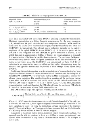
![214 HSDPA/HSUPA for UMTS
For plain voice services the number of blocked calls is an important indicator of how
the end user experiences network quality. The number of blocked calls may be computed
analytically by means of the well-known Erlang formulas. For data services, where
blocking does not occur, an analytical approach to quantify network quality is more
challenging. Instead, simulations are typically used to evaluate the performance of
cellular data services. To keep it simple the simulation approach taken here does not
consider radio interface properties in detail. Instead, the users in one cell are assumed to
share a bit pipe characterized by the following two properties:
. The throughput of the bit pipe is constant and independent of the number of users.
. The throughput of the bit pipe is shared equally between all users.
Note that with this simple model some well-known cellular effects – like lower bit rates at
the cell border than at the cell centre – are not considered. However, if we take the
average cell throughputs of Release 99 DCH and HSDPA from Chapter 7, then this
simple model already provides us with good insights into the load vs performance trade-
off for WCDMA/HSPA networks. Active browsing users are assumed to have the
following simplified usage pattern:
. Each active user downloads a 300-kB-large Internet page every second minute.
. Internet browsing is the only service used in the cell.
The page size of 300 kB is chosen to represent a medium-sized Internet page. The
download time of the Internet page is – in the simulations – computed by dividing
the page size by the instantaneous bit rate offered by the shared bit pipe. This approach
excludes effects like bearer setup times and rendering times and the download times from
the simulations are hence to be interpreted as best-case examples. In addition to the
active browsing users considered in the simulations, there may be a large number of
inactive users within the coverage area of one cell. These inactive users are not considered
in the simulations.
The simulation results are shown in Figure 9.26. Internet page download times are
given as functions of the number of active browsing users in the cell, and results for 1-, 2-,
and 4-Mbps-large bit pipes are shown. The average downlink cell throughput of a
Release 99 DCH cell can be close to 1 Mbps, while HSDPA improves the capacity to
2 Mbps with single-antenna terminals and up to 4 Mbps with advanced terminals.
Figure 9.26 shows that capacity is 50, 150, and 360 active browsing users per carrier
whenever end users are happy to wait the average 5 sec for a 300-kB Internet page. How
many browsing users may be supported per carrier depends heavily on the usage pattern.
When users download an Internet page every minute instead of every second minute,
then the number of supported users is 50% lower. Calculations show that HSDPA can
support a large number of browsing users. The number of users is higher than is the case
with WCDMA voice capacity, which is typically 60–130 users per cell [12].
It can also be observed from Figure 9.26 that the cell capacity in terms of the number of
browsing users triples when the maximum total cell throughput doubles from 1 to
2 Mbps. This shows that there is a 50% trunking gain available when increasing the
cell throughput from 1 to 2 Mbps. For the operator this means that three times as many](https://image.slidesharecdn.com/wileyhsdpahsupaforumts-12712250730845-phpapp02/85/Hsdpa-Hsupa-For-Umts-245-320.jpg)
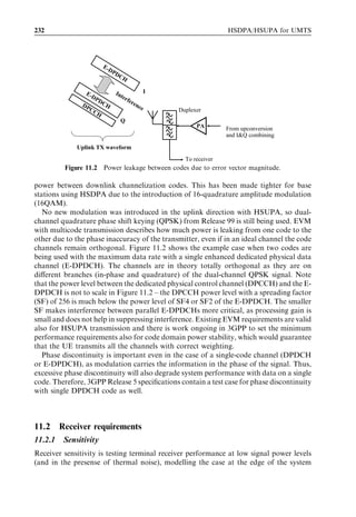
![216 HSDPA/HSUPA for UMTS
10
9 Maximum cell throughput: 2 Mbps
8 Theoretical download time
7
6
s 5
4
3
2
1
0
10 % 20 % 30 % 40 % 50 % 60 % 70 % 80 % 90 %
Load level
Figure 9.27 Average download time for a 300-kB Internet page as a function of load level.
this approach and by knowing the number of megabytes that each data user consumes on
average per month, it is straightforward to obtain a first understanding for how many
data users a HSDPA cell can support while still maintaining adequate service levels. This
calculation method is demonstrated in Section 7.5.
9.5 References
[1] ITU-T Recommendation G.114 (2003), One-way transmission time.
[2] ITU-T Recommendation P.800 (1996), Methods for subjective determination of transmis-
sion quality.
[3] 3GPP Technical Specification, TS 24.008, Mobile Radio Interface Layer 3 Specification,
Core Network Protocols, available at www.3gpp.org
[4] 3GPP Technical Specification, TS 25.331, Radio Resource Control (RRC), Protocol Spe-
cification, available at www.3gpp.org
[5] 3GPP Technical Specification, TS 25.433, UTRAN Iub interface Node B Application Part
(NBAP) Signalling, available at www.3gpp.org
[6] 3GPP Technical Specifications, TS 25.413, UTRAN Iu Interface Radio Access Network
Application Part (RANAP) Signalling, available at www.3gpp.org
[7] C. Johnson, H. Holma, and I. Sharp (2005), Connection setup delay for packet switched
services, IEE International Conference on 3G and Beyond (3G 2005), London, November.
[8] C. Johnson, R. Cuny, G. Davies, and N. Wimolpitayarat (2005), Inter-system handover for
packet switched services, IEE International Conference on 3G and Beyond (3G 2005),
London, November.
[9] OMA (Open Mobile Alliance), Push to Talk over Cellular Requirements, Version 1.0,
29 March 2005.
[10] Forum Nokia, Multiplayer Game Performance over Cellular Networks, Version 1.0,
20 January 2004.
[11] IETF RFC 2988, Computing TCP’s Retransmission Timer, November 2000.
[12] H. Holma and A. Toskala (2004) WCDMA for UMTS (3rd edn.). Wiley, Chichester, UK.](https://image.slidesharecdn.com/wileyhsdpahsupaforumts-12712250730845-phpapp02/85/Hsdpa-Hsupa-For-Umts-247-320.jpg)
![10
Voice-over-IP
Harri Holma, Esa Malkamaki, and Klaus Pedersen
¨
Voice over IP (VoIP) has turned out to be an attractive solution for carrying voice over
the packet-switched domain in the fixed network. A number of computer-based VoIP
clients are emerging (e.g., Skype [1]) which allow packet-based voice calls between
computers and handheld devices to be made over the public Internet. VoIP is also
emerging as an add-on feature to Internet Protocol (IP) applications like messaging
or netmeeting.
Wideband code division multiple access (WCDMA) and high-speed packet access
(HSPA) make it possible to carry good quality VoIP over wide area cellular networks as
well. The implementation of VoIP requires a proper understanding of VoIP radio
performance, but other aspects of VoIP also need to be considered including multi-
operator service level agreements, international roaming, termination fees, and regula-
tory aspects. This chapter focuses on the radio performance of VoIP. The main
motivations for running VoIP over cellular networks are discussed, IP header compres-
sion is introduced, and system capacity results are presented. The radio performance of
VoIP on Release 99 dedicated channels has previously been studied ([2]–[4]).
10.1 VoIP motivation
Circuit-switched voice has been the main source of revenue for cellular operators and still
constitutes 70% of their revenue. So far, cellular networks have not been able to
support good-quality voice over packet-switched channels, but with WCDMA/HSPA
radio performance will be good enough for VoIP. VoIP can be implemented either to
support rich call services or just because it will provide the same plain vanilla voice service
but with lower cost than traditional circuit-switched voice. This section briefly introduces
the different drivers necessary to run VoIP over WCDMA/HSPA and we differentiate
between the following three cases:
HSDPA/HSUPA for UMTS: High Speed Radio Access for Mobile Communications Edited by Harri Holma
and Antti Toskala © 2006 John Wiley Sons, Ltd. ISBN: 0-470-01884-4](https://image.slidesharecdn.com/wileyhsdpahsupaforumts-12712250730845-phpapp02/85/Hsdpa-Hsupa-For-Umts-248-320.jpg)
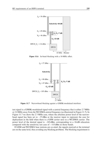
![Voice-over-IP 219
100 37.6 kbps
RLC header
90
RTP/UDP/IPv6 header
80
RTP payload AMR12.2 kbps
Bytes per 20-ms frame 70
60
50
15.2 kbps
40
30
20
10
0
Uncompressed headers ROHC
Figure 10.2 Benefit from robust IP header compression (ROHC) in 12.2-kbps VoIP.
justified for plain voice services if circuit-switched voice is not supported. A number of
other packet-based radio systems, including WLAN or Wimax, are not able to carry
circuit-switched voice. If the voice service is required over those radio systems, VoIP is
the only option – even for a simple voice service.
10.2 IP header compression
The size of a full IPv6 header together with a Real Time Protocol/User Datagram
Protocol (RTP/UDP) header is 60 bytes, while the size of a typical voice packet is
30 bytes. Without header compression two-thirds of the transmission would be just
headers. IP header compression can be applied to considerably improve the efficiency
of VoIP traffic in HSPA. We assume usage of robust header compression (ROHC),
which is able to push the size of the headers down to a few bytes [7]. ROHC in the Third
Generation Partnership Project (3GPP) is part of Release 4. Figure 10.2 illustrates the
required data rate with full headers and with compressed headers. The required data rate
is reduced from close to 40 kbps down to below 16 kbps.
Header compression with HSPA is done on the Layer 2 Packet Data Convergence
Protocol (PDCP) in the user equipment (UE) and in the radio network controller (RNC);
therefore, it saves not only air interface capacity but also Iub transmission capacity. The
header compression location is illustrated in Figure 10.3.
10.3 VoIP over HSPA
High-speed downlink/uplink packet access (HSDPA/HSUPA) was originally designed
for high bit rate non-real time services while VoIP is a low bit rate service with strict or](https://image.slidesharecdn.com/wileyhsdpahsupaforumts-12712250730845-phpapp02/85/Hsdpa-Hsupa-For-Umts-250-320.jpg)
![220 HSDPA/HSUPA for UMTS
Compressed IP headers Full IP headers
BTS RNC SGSN/GGSN
Iub
Header compression on PDCP layer
Figure 10.3 IP header compression with VoIP.
tough requirements. The simulation results in this section show, however, that 3GPP
HSPA can still provide an attractive performance for VoIP.
10.3.1 HSDPA VoIP
10.3.1.1 Packet scheduling and delay budget
HSDPA VoIP simulations assume proportional fair packet scheduling (for details see
Chapter 6). Code-multiplexing of users (Musers ) is assumed. The scheduler selects those
Musers with highest priority from the scheduling candidate set for transmission in the next
2-ms transmission time interval (TTI). The scheduling candidate set includes users that
fulfill the following criteria [6]:
1. Users that have at least Mpkts of VoIP packets buffered in the Node B. The value for
Mpkts depends on the maximum allowed VoIP delay and was between 3 and 4 in the
following simulations.
2. Users whose head-of-line packet delay is equal to or larger than ðMpkts À 1Þ Â 20 ms.
3. Users with pending retransmissions in their hybrid automatic repeat request (HARQ)
manager.
Using these criteria, we try to avoid scheduling users with low amounts of buffered data
in the Node B, which might cause a loss of system capacity. Note that a single VoIP
packet with ROHC is typically only 38 bytes or 304 bits while the HSDPA transport
block size with, say, three high-speed downlink shared channel (HS-DSCH) codes can be
clearly beyond 1500 bits. Therefore, a single transport block can carry multiple VoIP
packets.
According to the International Telecommunication Union (ITU) model [7], one-way
mouth-to-ear delay should be less than 250 ms to achieve a good to acceptable voice
quality rating. We estimate that the available VoIP packet delay budget for Node B
scheduling, air–interface transmission, and UE reception roughly equals 80–150 ms,
depending on whether the VoIP call is between two mobiles or between a land-line
and a mobile user.](https://image.slidesharecdn.com/wileyhsdpahsupaforumts-12712250730845-phpapp02/85/Hsdpa-Hsupa-For-Umts-251-320.jpg)
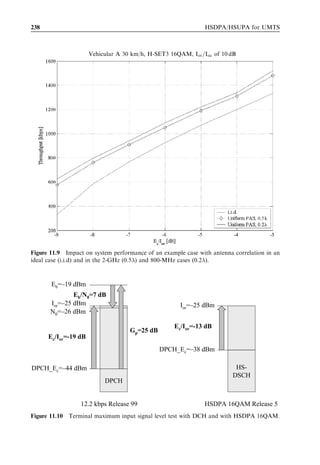
![222 HSDPA/HSUPA for UMTS
transmission, a clear improvement over only 10 codes with a 3GPP Release 5 associated
DCH. When more HS-PDSCH codes are available, stronger channel coding and more
robust modulation can be applied, thus improving spectral efficiency.
In terms of power allocations the simulations assume that common channels take 3 W,
associated DCHs 1 W, the HS-SCCHs 2 W and the HS-DSCH 10 W, leading to
an average Node B power of 16 W, which leaves some room for fluctuations in associated
DCH power levels.
10.3.1.3 Capacity results
The downlink network simulator described in [6] has been used to investigate the
performance of VoIP on HSDPA. Each newly arrived VoIP packet in the Node B is
associated with a discard timer. Whenever a buffered packet has been transmitted, it is
moved to the HARQ manager and its discard timer is de-activated. Hence, whenever a
packet has been transmitted, it can be dropped only if it has not been successfully
received after the maximum number of allowed transmissions. For more details of
the simulator, see [6].
Figure 10.5 shows the macro-cell simulation results with different delay values for
transmission from the RNC to the UE’s play-out buffer. The maximum capacity with
80-ms, 100-ms, and 150-ms maximum delays is 73, 87, and 105 users with 5% cell outage.
There is clearly a trade-off between delay and capacity with VoIP: if more delay can be
tolerated, voice capacity increases.
These VoIP capacity figures can be compared with the estimated Release 99 voice
capacity of 64 users [8]. HSDPA can improve voice capacity as a result of advanced L1
0.08
0.07
80 ms
delay
budget 100 ms 150 ms
Cell outage probability
0.06 delay delay
budget budget
0.05
0.04
0.03
0.02
65 70 75 80 85 90 95 100 105 110
Average number of VoIP users per cell
Figure 10.5 Cell outage probability for VoIP for different delay budgets.](https://image.slidesharecdn.com/wileyhsdpahsupaforumts-12712250730845-phpapp02/85/Hsdpa-Hsupa-For-Umts-253-320.jpg)
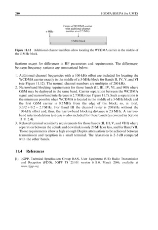
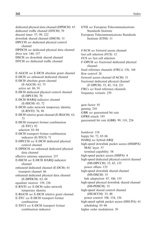
![226 HSDPA/HSUPA for UMTS
VA3, with HS-DPCCH
8
7
6
5
Noise rise (dB)
4
3
10 ms TTI, 80% throughput
2 2 ms TTI, 50% throughput
10 ms TTI, 60% throughput
1 2 ms TTI, 33% throughput
0
30 40 50 60 70 80 90 100 110 120
Number of VoIP users
Figure 10.9 Uplink noise rise as a function of number of VoIP users for different TTI lengths and
single-user throughputs in the Vehicular A channel using a 3-km/h channel.
for downlink power control. When no data are transmitted between VoIP packets, no
channel estimation is needed either. Possibilities for gating DPCCH transmission when
there is no other uplink transmission are being studied in 3GPP for Release 7. The target
is to reduce interference and improve capacity. HSUPA uplink capacity is addressed in
3GPP [9].
The spectral efficiency gain from HSUPA can be achieved with several retransmis-
sions. Each retransmission needs to be decoded by the Node B receiver, and the Node B
baseband needs to be dimensioned with twice to three times as much processing power
than is the case where the number of retransmissions is kept small.
10.3.3 Capacity summary
HSDPA and HSUPA VoIP simulation results are summarized in Figure 10.10. HSDPA
results are based on 3GPP Release 5 with an associated DCH, single-antenna Rake
receiver, and a maximum 80-ms transmission delay. HSUPA results are based on 3GPP
Release 6 with a maximum 60-ms transmission delay. Achieved capacity in the downlink
and uplink is similar to WCDMA circuit-switched voice capacity.
HSDPA capacity can be increased by using a fractional DPCH and the advanced
terminal receivers that are part of 3GPP Release 6. HSUPA capacity can be increased
with 3GPP Release 7 based gating. When all these enhancements are included, VoIP
capacity is expected to exceed 120 users with an adaptive multi-rate (AMR) 12.2-kbps
codec.](https://image.slidesharecdn.com/wileyhsdpahsupaforumts-12712250730845-phpapp02/85/Hsdpa-Hsupa-For-Umts-257-320.jpg)
![Voice-over-IP 227
160
Advanced UE and Uplink gating Uplink gating
fractional DPCH (expected for (expected for
140
(3GPP R6) 3GPP R7) 3GPP R7)
120
Users per sector
100
80
60
40
20
0
Downlink 1-Rake Uplink 10-ms TTI Uplink 2-ms TTI
(3GPP R5) (3GPP R6) (3GPP R6)
Figure 10.10 Summary of VoIP capacity results for an AMR of 12.2 kbps.
10.4 References
[1] www.skype.com
[2] F. Poppe, D. de Vleeschauwer, and G. H. Petit (2000), Guaranteeing quality of service to
packetized voice over the UMTS air interface, Eighth International Workshop on Quality of
Service, June, pp. 85–91.
[3] F. Poppe, D. de Vleeschauwer, and G. H. Petit (2001), Choosing the UMTS air interface
parameters, the voice packet size and the dejittering delay for a voice-over-ip call between a
umts and a pstn party, IEEE INFOCOM, 2, 805–814, April.
[4] R. Cuny and A. Lakaniemi (2003), VoIP in 3G networks: An end-to-end quality of service
analysis, IEEE Proc. Vehicular Technology Conference, Spring, Vol. 2, pp. 930–934.
[5] IETF RFC 3095, Robust Header Compression (ROHC), Framework and four profiles:
RTP, UDP, ESP, and uncompressed, July 2001.
[6] W. Bang, K. I. Pedersen, T. E. Kolding, and P. E. Mogensen (2005), Performance of VoIP
on HSDPA, IEEE Proc. Vehicular Technology Conference, Stockholm, June.
[7] ITU, One Way Transmission Time, ITU-T Recommendation G.114.
[8] H. Holma and A. Toskala (eds) (2004), WCDMA for UMTS (3rd edn), John Wiley Sons,
Chichester, UK.
[9] 3GPP Technical Report, TR 25.903, Continuous Connectivity for Packet Data Users,
Release 7.](https://image.slidesharecdn.com/wileyhsdpahsupaforumts-12712250730845-phpapp02/85/Hsdpa-Hsupa-For-Umts-258-320.jpg)
![11
RF requirements of an
HSPA terminal
Harri Holma, Jussi Numminen, Markus Pettersson, and Antti Toskala
This chapter presents the principal parts of a Third Generation Partnership Project
(3GPP) terminal’s radio frequency (RF) performance requirements with an emphasis on
the new aspects introduced using high-speed downlink/uplink packet access (HSDPA/
HSUPA). Section 11.1 presents the transmitter requirements and Section 11.2 the
receiver requirements. The different frequency bands are introduced in Section 11.3.
For detailed requirements, the reader is referred to [1].
11.1 Transmitter requirements
11.1.1 Output power
Commercial wideband code division multiple access (WCDMA) and HSDPA terminals
are Power Class 3 with 24 dBm maximum output power or Power Class 4 with 21 dBm
power. Power Class 4 has a tolerance of þ1/À3 dB – that is, terminal output power must
be in the range of 21–25 dBm. Tolerance in Power Class 3 is þ2/À2 dB. If terminal output
power is 22 dBm, the terminal could be classified either as a Class 3 or a Class 4 terminal
due to the overlap in class definition. The power classes are summarized in Table 11.1.
Higher terminal output power can improve uplink data rates in the weak coverage area.
HSDPA introduces a new uplink channel for L1 feedback called the ‘high-speed
dedicated physical control channel’ (HS-DPCCH). The transmission of HS-DPCCH
Table 11.1 UE power classes.
Power Class 3 Power Class 4
Maximum power þ24 dBm þ21 dBm
Tolerance þ1/À3 dB þ2/À2 dB
HSDPA/HSUPA for UMTS: High Speed Radio Access for Mobile Communications Edited by Harri Holma
and Antti Toskala © 2006 John Wiley Sons, Ltd. ISBN: 0-470-01884-4](https://image.slidesharecdn.com/wileyhsdpahsupaforumts-12712250730845-phpapp02/85/Hsdpa-Hsupa-For-Umts-259-320.jpg)


