Reviewing Probability Distributions Doing stats with python way

1. Reviewing Probability Distributions
A probability distribution is a mathematical function that describes the
likelihood of different outcomes for a random variable.
It essentially shows the spread and shape of a dataset, allowing us to
understand and predict the probability of events.
Probability distributions are categorized as discrete or continuous, depending
on whether the random variable can take on a finite or infinite number of
values, respectively.
A Probability Distribution of a random variable is a list of all possible outcomes
with corresponding probability values.

2. Key Concepts:
Random Variable:
A variable whose value is a numerical outcome of a random phenomenon.
(Number of balls in a bag, number of tails in tossing coin)
Probability:
A measure of the likelihood of an event occurring, ranging from 0 (impossible) to 1 (certain).
(Flipping of two coins)
Probability Distribution Function (PDF):
For continuous distributions, the PDF gives the probability density for each possible value of the
random variable.
Cumulative Distribution Function (CDF):
For any distribution, the CDF gives the probability that the random variable is less than or equal to
a given value.
Discrete vs. Continuous Distributions:
Discrete distributions deal with countable outcomes (e.g., number of heads in coin flips), while
continuous distributions deal with outcomes that can take any value within a range (e.g., height,
weight).

3. Common Types of Probability Distributions:
Binomial Distribution: Models the probability of a certain number of successes in a fixed
number of independent trials, each with the same probability of success.
P(x:n,p) = nCx px (1-p)n-x
Or
P(x:n,p) = nCx px (q)n-x
If a coin is tossed 5 times, find the probability of:
Exactly 2 heads
The repeated tossing of the coin is an example of a Bernoulli trial. According to the
problem:
Number of trials: n=5
Probability of head: p= 1/2 and hence the probability of tail, q =1/2
For exactly two heads: x=2
P(x=2) = 5C2 p2 q5-2 = 5! / 2! 3! × (½)2× (½)3
P(x=2) = 5/16

4. Normal Distribution: A bell-shaped, symmetrical distribution that is
widely used in statistics.
The probability density function of normal or gaussian distribution is
given by;
Normal Distribution Formula
Where,
x is the variable
μ is the mean
σ is the standard deviation
Exponential Distribution: Models the time until an event occurs.

5. Example:Time Until an Event:
Customer Service: The time between customer arrivals at a bank or a store.
Manufacturing: The time until a machine part fails.
Telecommunications: The duration of phone calls.
Web Servers: The time between requests.
Accidents: The time until an accident at a manufacturing plant.
Assume that, you usually get 2 phone calls per hour. calculate the probability, that a phone call will come
within the next hour.
Solution:
It is given that, 2 phone calls per hour. So, it would expect that one phone call at every half-an-hour. So,
we can take
λ = 0.5
So, the computation is as follows:
P(0<=X<=1)=Sum(0.5e-0.5x)
= 0.393469
Therefore, the probability of arriving the phone calls within the next hour is 0.393469

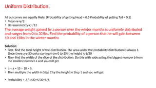
6. Uniform Distribution:
All outcomes are equally likely. (Probability of getting Head = 0.5 Probability of getting Tail = 0.5)
• Mean=x+y/2
• SD=suareroot(y-x)2
/12
The average weight gained by a person over the winter months is uniformly distributed
and ranges from 0 to 30 lbs. Find the probability of a person that he will gain between
10 and 15lbs in the winter months
Solution:
• First, find the total height of the distribution. The area under the probability distribution is always 1.
Since there are 30 units starting from 0 to 30) the height is 1/30
• Then find the width of the slice of the distribution. Do this with subtracting the biggest number b from
the smallest number a and you will get
• b – a = 15 – 10 = 5.
• Then multiply the width in Step 2 by the height in Step 1 and you will get
• Probability = .5*1/30=5/30=1/6

7. Poisson Distribution: Models the probability of a certain number of
events occurring within a fixed interval of time or space.
Let in a hospital patient arriving in a hospital at expected value is 6,
then what is the probability of five
patients will visit the hospital in that day?
Patients arriving at expected value = 6
P(Five patients will visit the hospital) = P(X = 5)
P(X=5)=65
e6
/5!
0.1606

8. Applications:
Probability distributions are fundamental in statistics and data science,
enabling us to:
Analyze data: Understand the characteristics and patterns of data.
Make predictions: Estimate the likelihood of future events.
Model real-world phenomena: Represent and understand various
situations, from stock prices to disease outbreaks.
Example:
• Imagine rolling a fair six-sided die. The probability of each outcome (1,
2, 3, 4, 5, or 6) is 1/6. This is a discrete uniform distribution.

9. Recollecting statistical measures
Statistical measures are tools used in descriptive statistics to summarize
and understand the characteristics of a dataset.
They provide concise descriptions of the data, including where its
center lies and how spread out the values are.
These measures are essential for gaining insights from data and forming
a foundation for further analysis or decision-making

10. 1. Measures of central tendency
These measures identify the central or typical value within a dataset.
The most common are:
Mean: The average of all values, calculated by summing all data points
and dividing by the number of values.
Median: The middle value when the data is ordered from smallest to
largest. It's less affected by outliers than the mean.
Mode: The value that appears most frequently in the dataset. A dataset
can have multiple modes or no mode at all.

11. 2. Measures of variability
These measures describe how spread out the data points are from each
other and from the center of the distribution.
Range: The difference between the highest and lowest values in the
dataset. It's a simple but sensitive measure as it relies on only two
values.
Interquartile Range (IQR): The range of the middle 50% of the data. It's
calculated as the difference between the third quartile (Q3) and the
first quartile (Q1) and is less affected by outliers than the range.
Variance: The average of the squared differences from the mean. It
provides a more comprehensive picture of variability than the range.
Standard Deviation: The square root of the variance. It's the most
common measure of variability as it's expressed in the same units as
the original data and is particularly useful for normally distributed data.

12. 3. Other descriptive measures
Skewness: Describes the asymmetry of a dataset's distribution.
A positive skew means a longer tail on the right, while a negative skew indicates a longer
tail on the left.
It measures how much a data set deviates from a symmetrical bell curve (normal
distribution).
Kurtosis: Measures the "tailedness" of a distribution, indicating whether it has heavier or
lighter tails than a normal distribution. Tailedness is how often outliers occur.
Correlation Coefficient: Measures the strength and direction of the linear relationship
between two variables. Pearson's correlation coefficient quantifies this relationship. A
correlation coefficient is a numerical measure of some type of linear correlation, meaning
a statistical relationship between two variables.