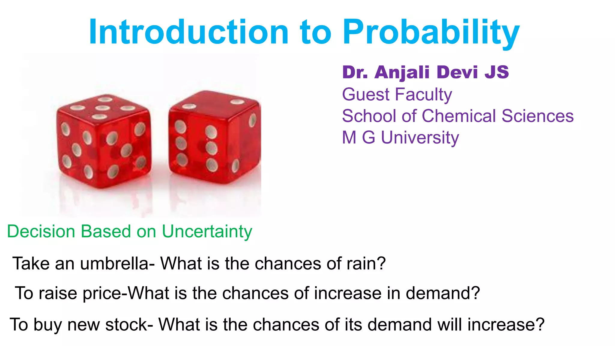
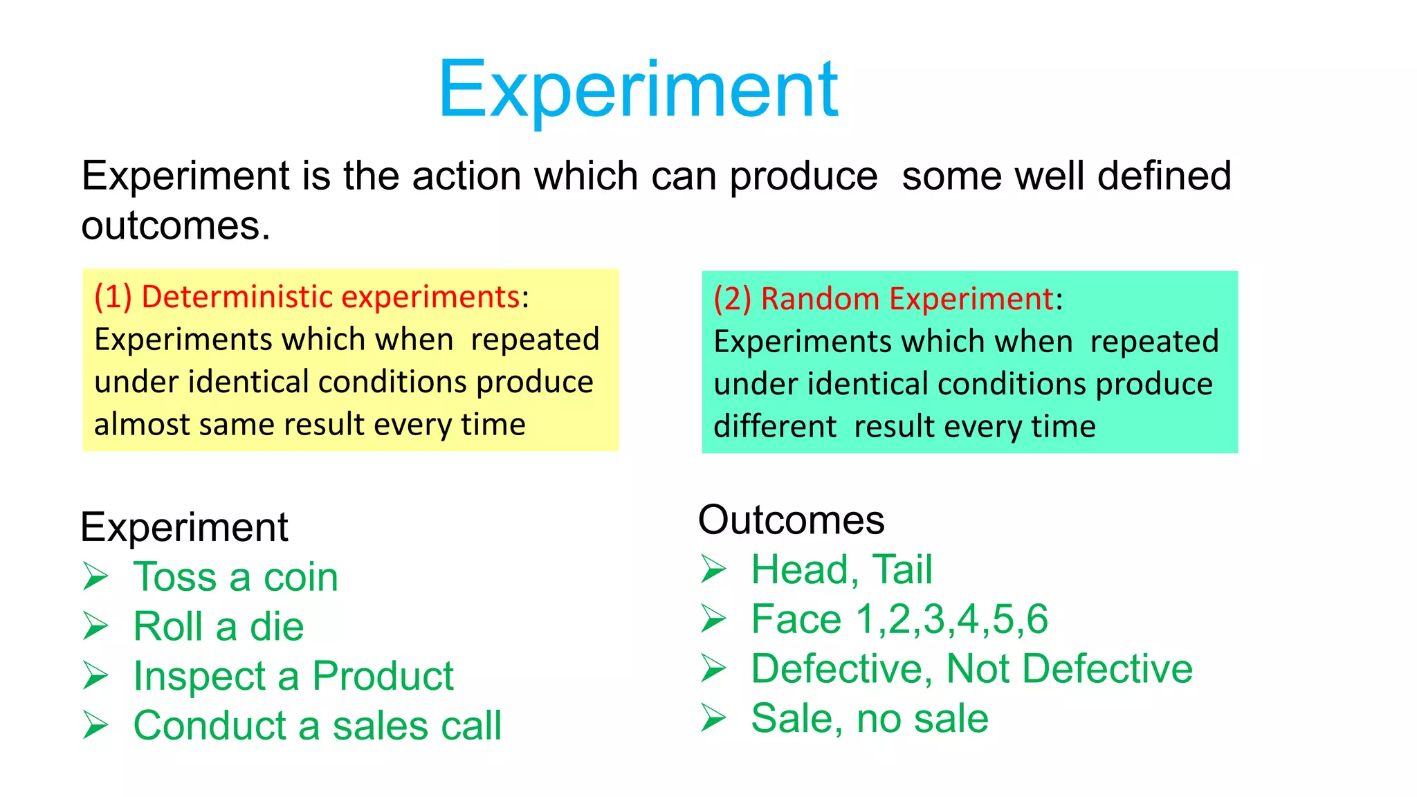
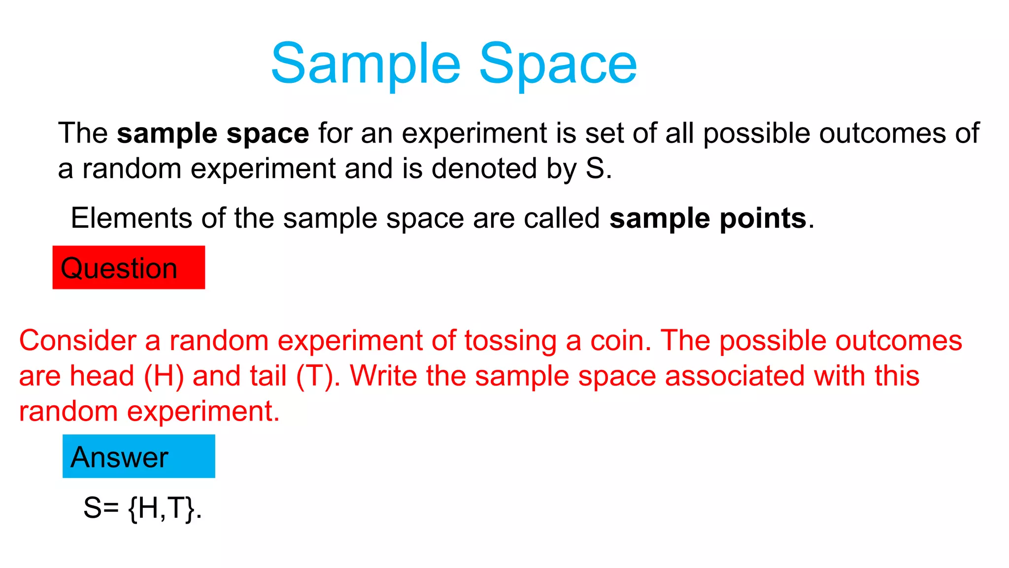
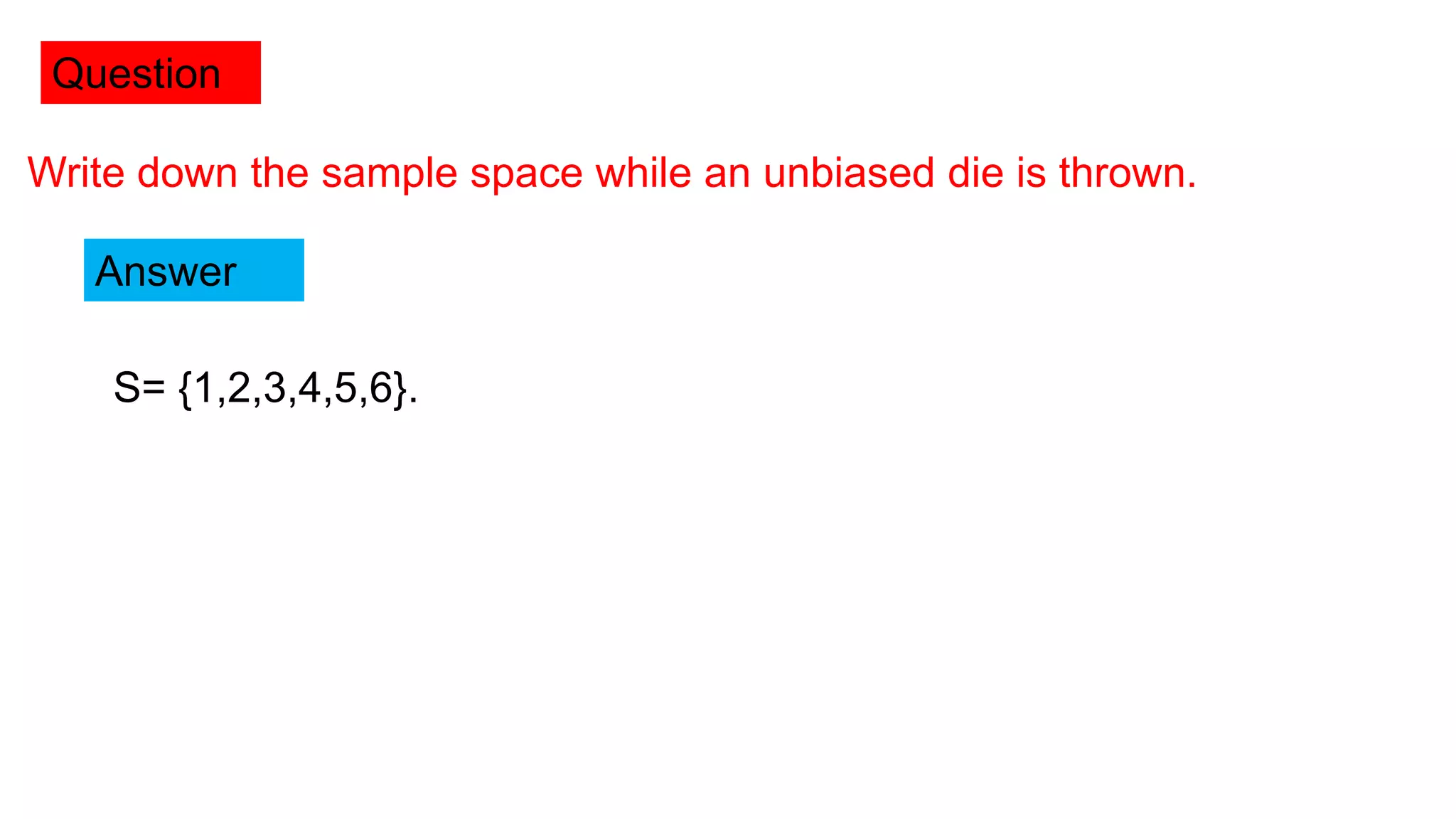
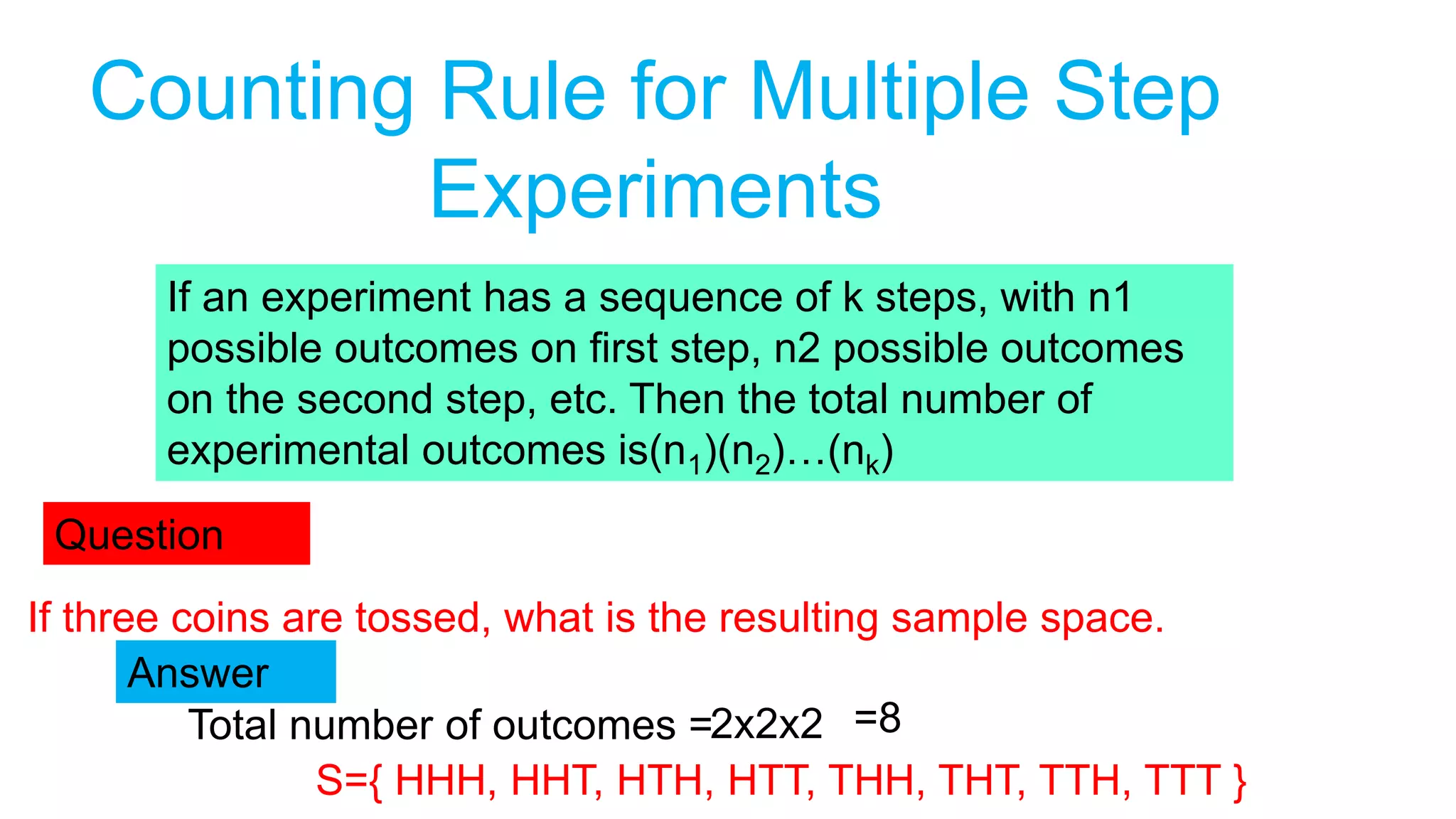
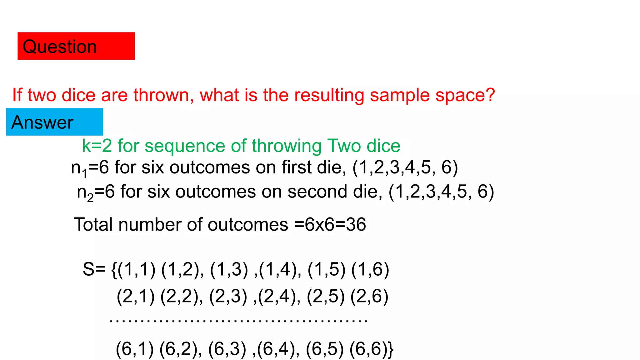
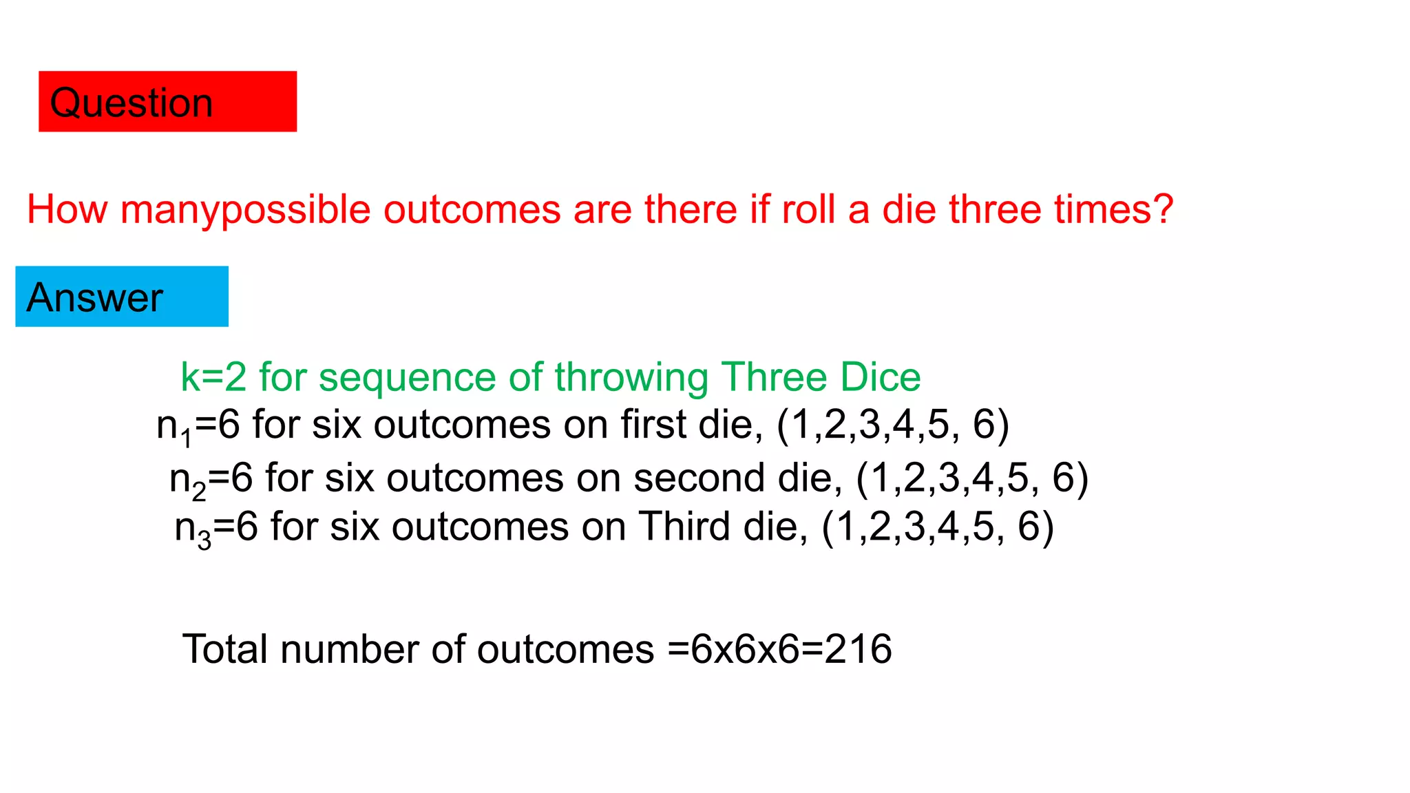
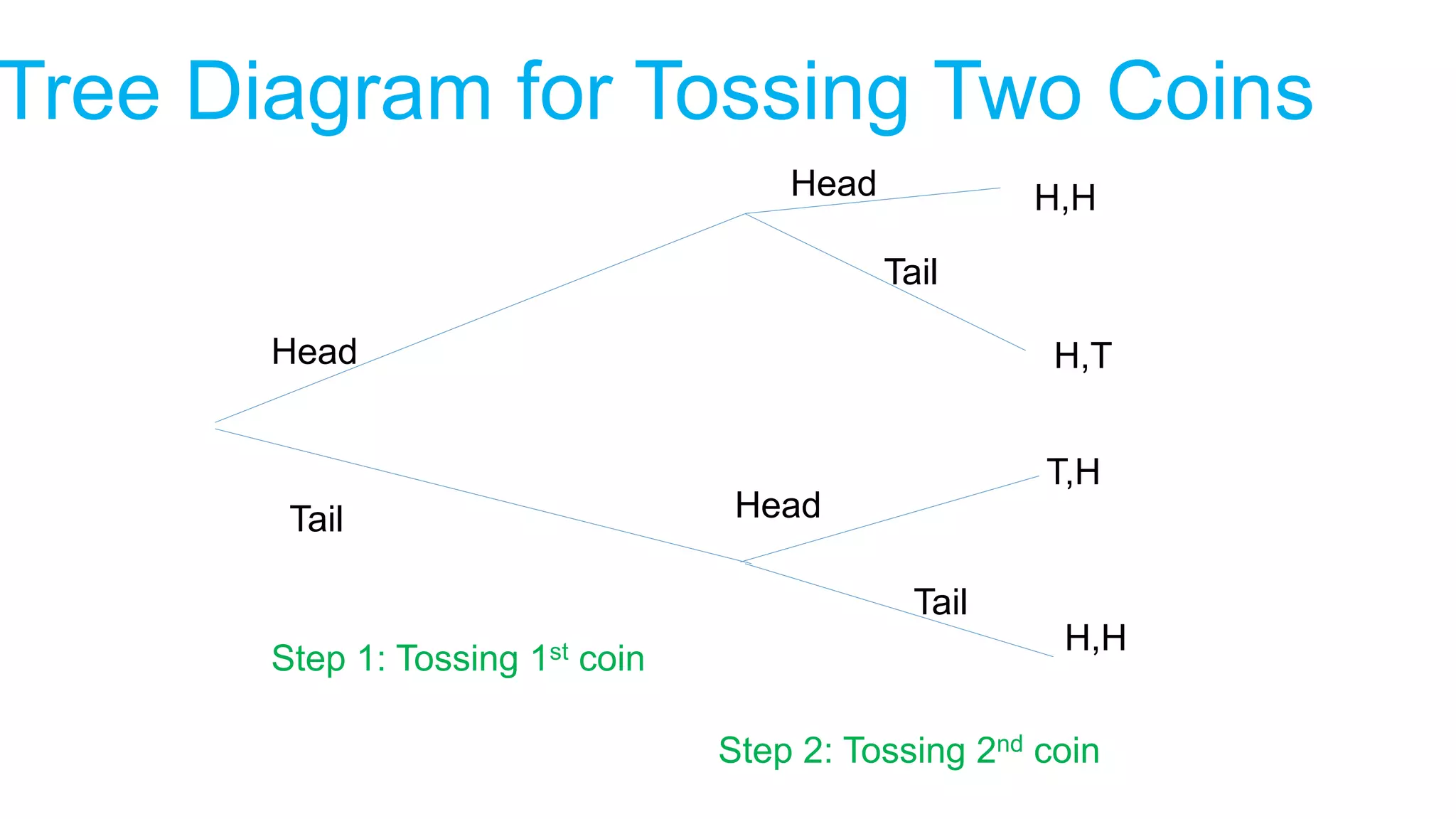
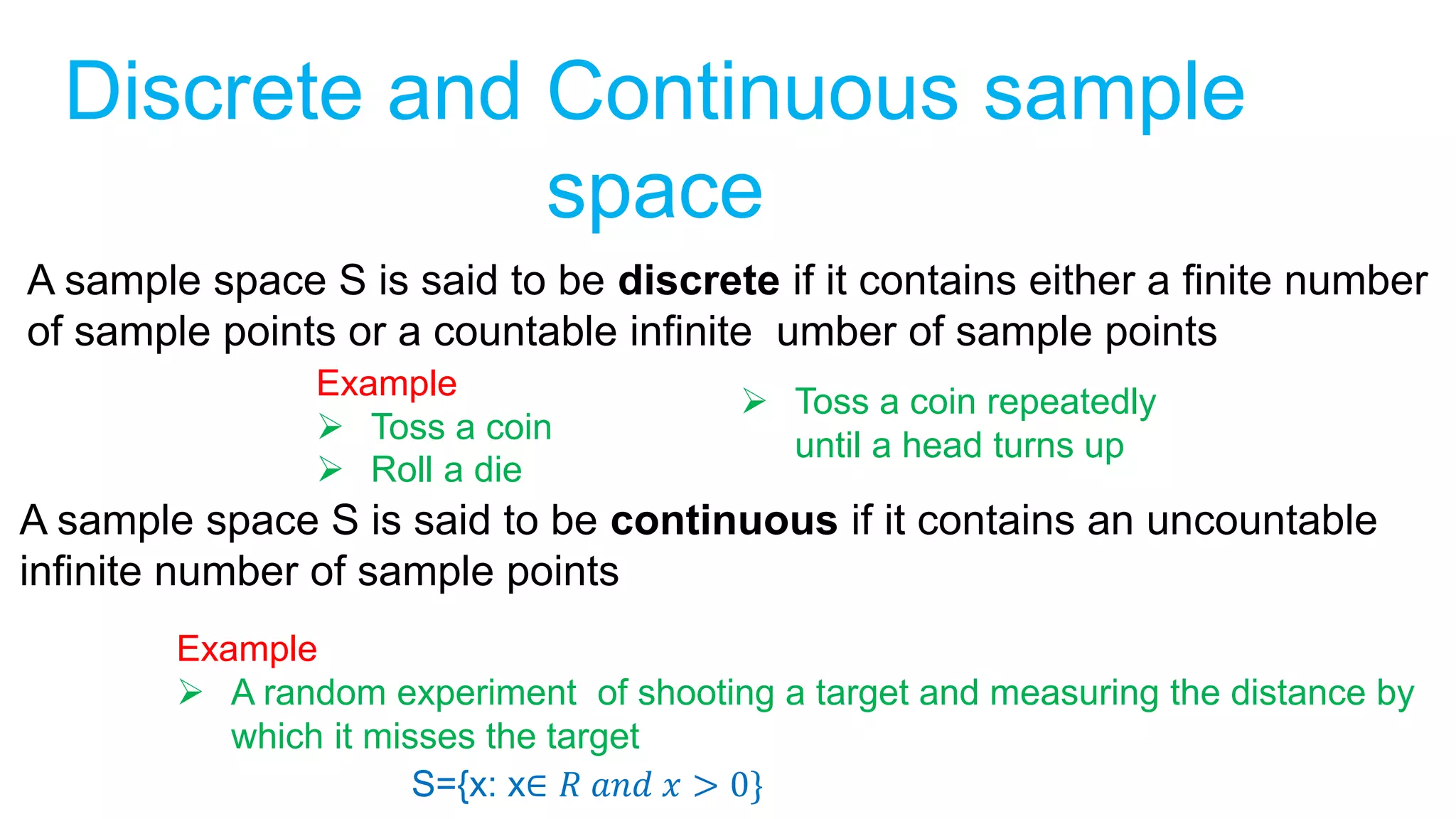
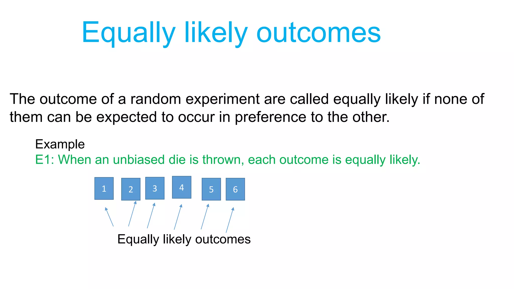
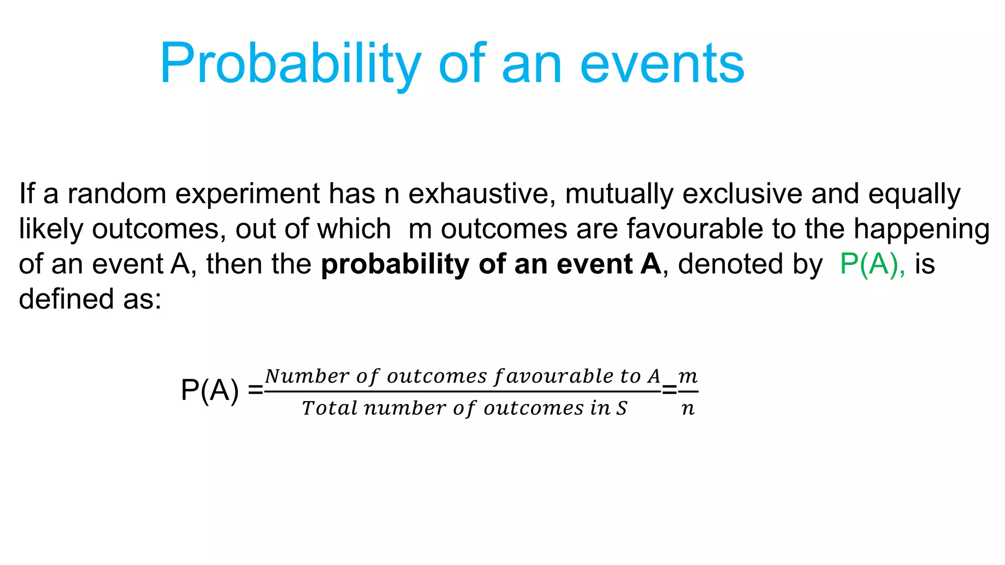
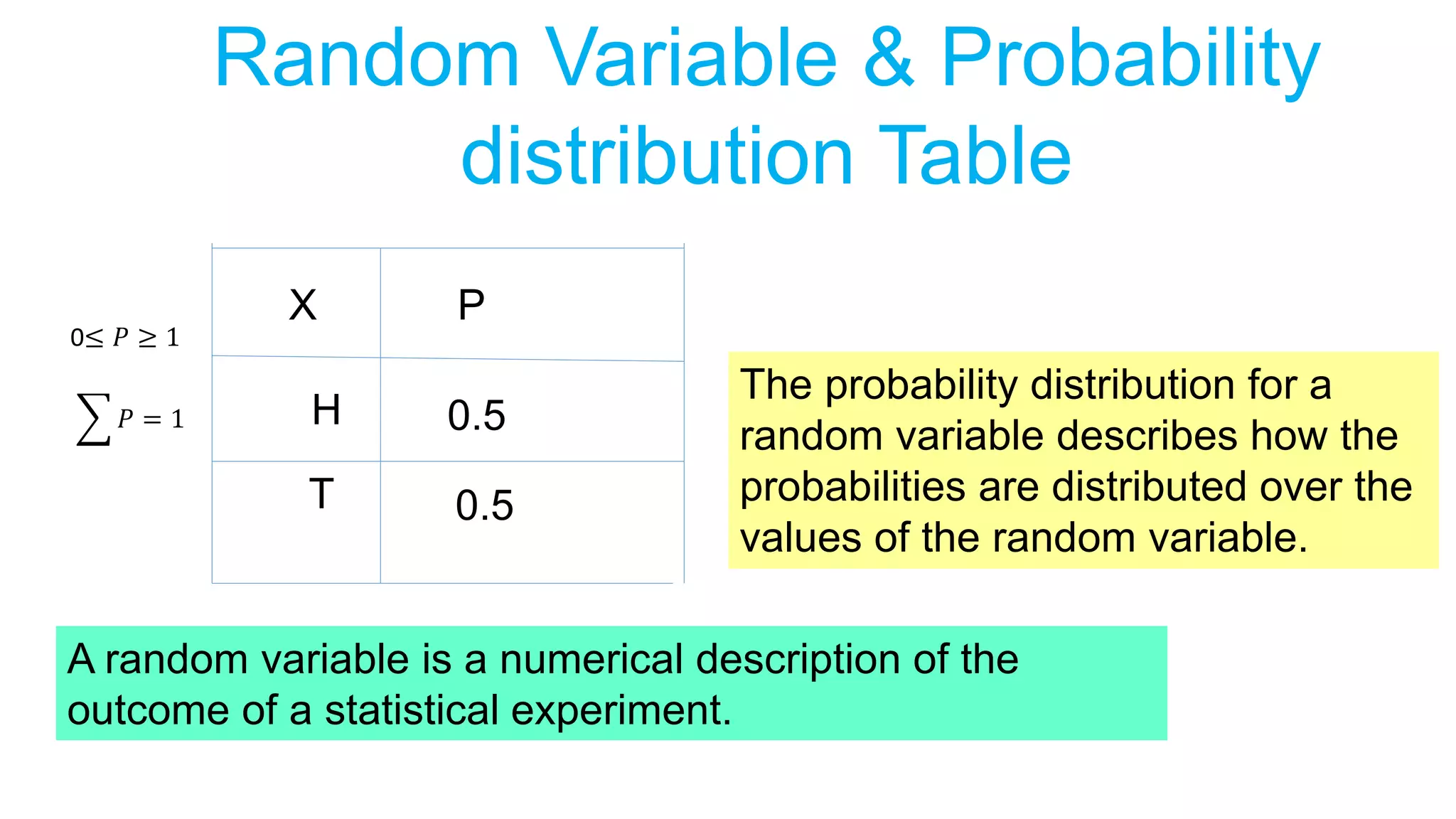
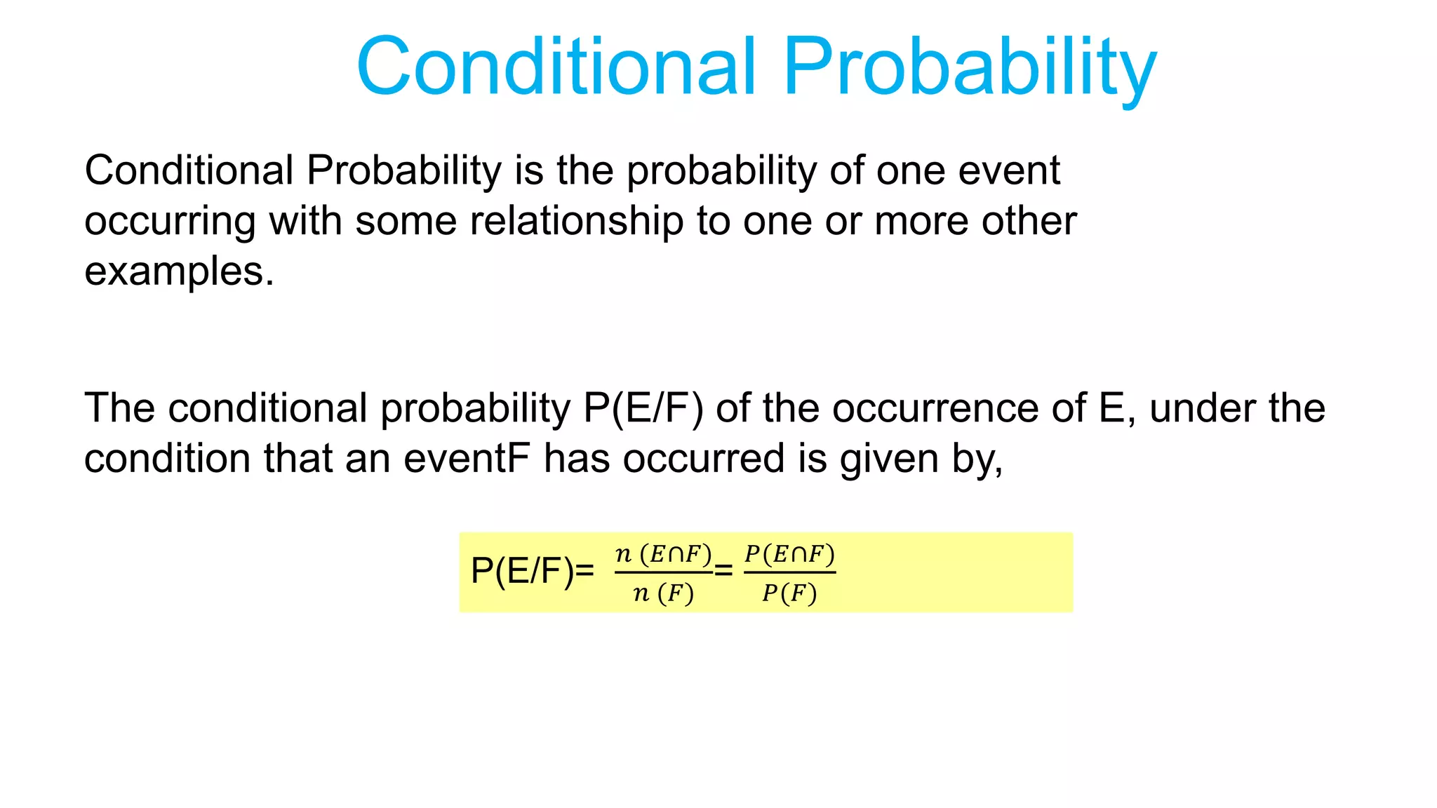
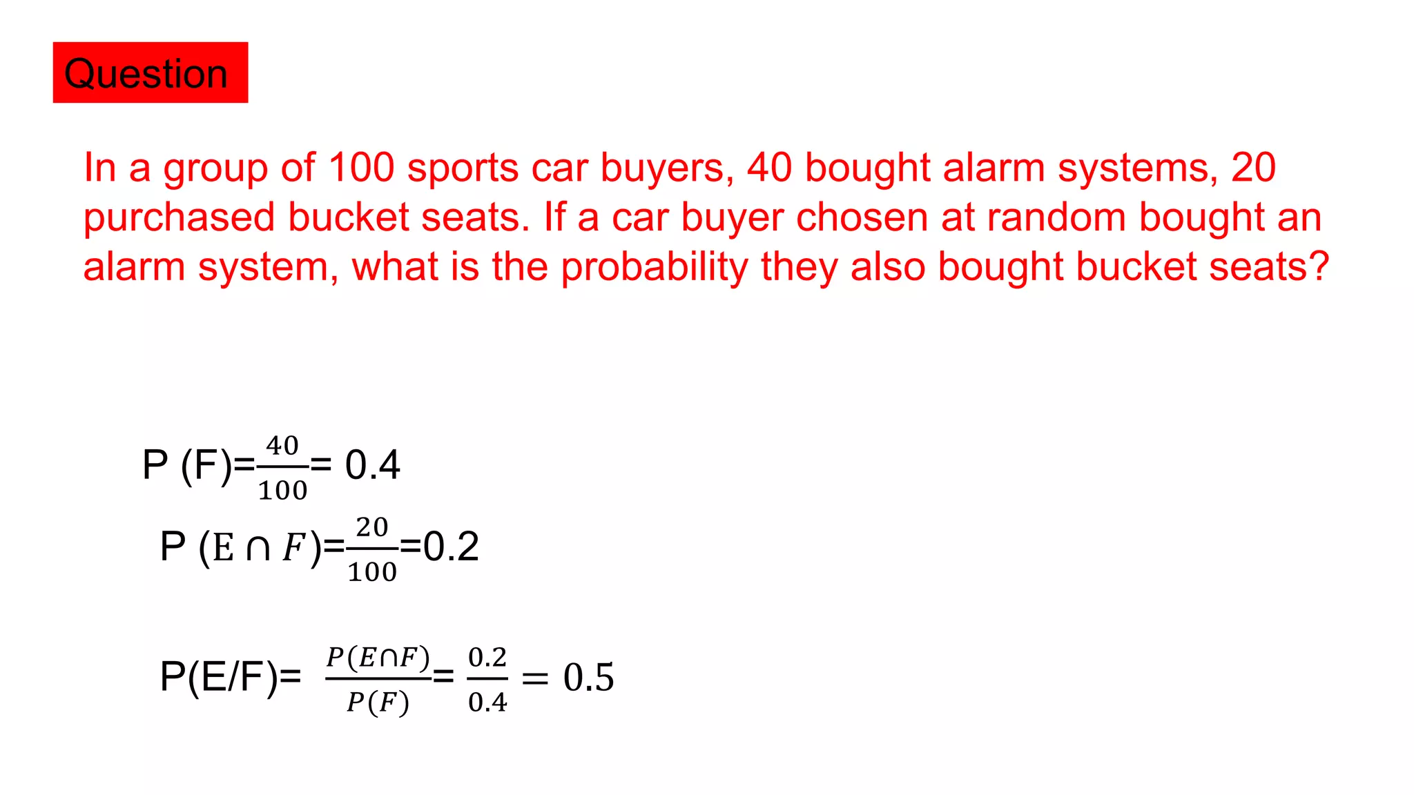
Probability is a numerical measure of how likely an event is to occur. It is defined as the number of favorable outcomes divided by the total number of possible outcomes. A random experiment is an action with some defined outcomes that may occur by chance. The sample space is the set of all possible outcomes. Conditional probability is the probability of one event occurring given that another event has occurred.

1. Introduction to Probability
Decision Based on Uncertainty
Take an umbrella- What is the chances of rain?
To raise price-What is the chances of increase in demand?
To buy new stock- What is the chances of its demand will increase?
Dr. Anjali Devi JS
Guest Faculty
School of Chemical Sciences
M G University

2. Probability
Probability is the numerical measure of likelihood that an event will
occur.
0 1.0
0.5
Increasing Likelihood
Event is just as likely
to occur as it is
unlikely to occur

3. Experiment
Experiment is the action which can produce some well defined
outcomes.
Experiment
 Toss a coin
 Roll a die
 Inspect a Product
 Conduct a sales call
Outcomes
 Head, Tail
 Face 1,2,3,4,5,6
 Defective, Not Defective
 Sale, no sale
(1) Deterministic experiments:
Experiments which when repeated
under identical conditions produce
almost same result every time
(2) Random Experiment:
Experiments which when repeated
under identical conditions produce
different result every time

4. Sample Space
The sample space for an experiment is set of all possible outcomes of
a random experiment and is denoted by S.
Elements of the sample space are called sample points.
Question
Consider a random experiment of tossing a coin. The possible outcomes
are head (H) and tail (T). Write the sample space associated with this
random experiment.
Answer
S= {H,T}.

5. Question
Suppose two fair coins are tossed. The following four outcomes are
possible.
Answer
S= {HH,HT, TH,TT}.
Sl No Outcomes Notation
(i) Head on first coin, head on second coin HH
(ii) Head on first coin, tail on second coin HT
(iii) Tail on first coin, head on second coin TH
(iv) Tail on first coin, tail on second coin TT
Write the sample space associated with this random experiment.

6. Question
Write down the sample space while an unbiased die is thrown.
Answer
S= {1,2,3,4,5,6}.

7. Counting Rule for Multiple Step
Experiments
If an experiment has a sequence of k steps, with n1
possible outcomes on first step, n2 possible outcomes
on the second step, etc. Then the total number of
experimental outcomes is(n1)(n2)…(nk)
Question
If three coins are tossed, what is the resulting sample space.
Total number of outcomes =2x2x2 =8
S={ HHH, HHT, HTH, HTT, THH, THT, TTH, TTT }
Answer

8. Question
If two dice are thrown, what is the resulting sample space?
Answer
k=2 for sequence of throwing Two dice
n1=6 for six outcomes on first die, (1,2,3,4,5, 6)
n2=6 for six outcomes on second die, (1,2,3,4,5, 6)
Total number of outcomes =6x6=36
S= {(1,1) (1,2), (1,3) ,(1,4), (1,5) (1,6)
(2,1) (2,2), (2,3) ,(2,4), (2,5) (2,6)
……………………………………
(6,1) (6,2), (6,3) ,(6,4), (6,5) (6,6)}

9. Question
How manypossible outcomes are there if roll a die three times?
Answer
k=2 for sequence of throwing Three Dice
n1=6 for six outcomes on first die, (1,2,3,4,5, 6)
n2=6 for six outcomes on second die, (1,2,3,4,5, 6)
n3=6 for six outcomes on Third die, (1,2,3,4,5, 6)
Total number of outcomes =6x6x6=216

10. Tree Diagram for Tossing Two Coins
Head
Tail
Step 1: Tossing 1st coin
Step 2: Tossing 2nd coin
Head
Tail
H,H
H,T
T,H
H,H
Head
Tail

11. Discrete and Continuous sample
space
A sample space S is said to be discrete if it contains either a finite number
of sample points or a countable infinite umber of sample points
Example
 Toss a coin
 Roll a die
 Toss a coin repeatedly
until a head turns up
A sample space S is said to be continuous if it contains an uncountable
infinite number of sample points
Example
 A random experiment of shooting a target and measuring the distance by
which it misses the target
S={x: x∈ 𝑅 𝑎𝑛𝑑 𝑥 > 0}

12. Events
Any subset of sample space is called an event.
Example
 Getting head when a coin is tossed
 Getting an odd number when a die is thrown
Each element of the sample space associated with a random
experiment is called an elementary event or simple event.
Example
Six elementary events of random experiment of throwing a die are
{1}, {2}. {3}, {4}, {5}, {6}.

13. Sure Event and Impossible Event
An event which is sure to occur is called a sure event and an event which
can never occur is called an impossible event.
Example of sure event
 Event of getting number less than 7 (when a
fair die is thrown)
Example of impossible event
 Event of getting number greater than 7 (when a
fair die is thrown)

14. Mutually exclusive events
Two events associated with a random experiment are said to be mutually
exclusive if the occurrence of one prevents the possibility of the
occurrence of the other.
Example
E1: Event of getting an even number when an unbiased die is
thrown.
E2: Event of getting an odd number when an unbiased die is
thrown.
E1 and E2 are mutually exclusive events.

15. Exhaustive events
A set of event is said to be exhaustive if they include all the possible
outcomes of the random experiment.
Example
E1: Event of getting a number less than 4 when an unbiased die
is thrown.
E2: Event of getting a number greater than 2 when an unbiased
die is thrown.
E1 and E2 are exhaustive events.

16. Equally likely outcomes
The outcome of a random experiment are called equally likely if none of
them can be expected to occur in preference to the other.
Example
E1: When an unbiased die is thrown, each outcome is equally likely.
1 2 3 4 5 6
Equally likely outcomes

17. Probability of an events
If a random experiment has n exhaustive, mutually exclusive and equally
likely outcomes, out of which m outcomes are favourable to the happening
of an event A, then the probability of an event A, denoted by P(A), is
defined as:
P(A) =
𝑁𝑢𝑚𝑏𝑒𝑟 𝑜𝑓 𝑜𝑢𝑡𝑐𝑜𝑚𝑒𝑠 𝑓𝑎𝑣𝑜𝑢𝑟𝑎𝑏𝑙𝑒 𝑡𝑜 𝐴
𝑇𝑜𝑡𝑎𝑙 𝑛𝑢𝑚𝑏𝑒𝑟 𝑜𝑓 𝑜𝑢𝑡𝑐𝑜𝑚𝑒𝑠 𝑖𝑛 𝑆
=
𝑚
𝑛

18. Question
Find the probability of:
(i) getting a tail when a coin is tossed
(ii) Getting a head when a coin is tossed
Answer S={H, T}
(i) Let A={T}
P(A) =
𝑁𝑢𝑚𝑏𝑒𝑟 𝑜𝑓 𝑜𝑢𝑡𝑐𝑜𝑚𝑒𝑠 𝑓𝑎𝑣𝑜𝑢𝑟𝑎𝑏𝑙𝑒 𝑡𝑜 𝐴
𝑇𝑜𝑡𝑎𝑙 𝑛𝑢𝑚𝑏𝑒𝑟 𝑜𝑓 𝑜𝑢𝑡𝑐𝑜𝑚𝑒𝑠 𝑖𝑛 𝑆
=
1
2
= 0.5
(ii) Let B={H}
P(B) =
1
2
= 0.5

19. Random Variable & Probability
distribution Table
X
H
T
P
0.5
0.5
0≤ 𝑃 ≥ 1
𝑃 = 1
A random variable is a numerical description of the
outcome of a statistical experiment.
The probability distribution for a
random variable describes how the
probabilities are distributed over the
values of the random variable.

20. Discrete & Continuous Random
variable
A random variable that may assume only a finite number
or infinite sequence of values is said to be discrete.
A random variable that may assume any value in some
interval on the real number line is said to be continuous.
Example: A random variable representing a number of
automobiles sold at a particular dealership on one day.
Example: A random variable representing the weight of a
person in kilograms.

21. Probability Distribution
For a discrete random variable, x, the probability
distribution is defined by probability mass function f(x).
The function provide the probability for each value of the
random variable.
For a continuous random variable, x, the probability
distribution is defined by probability density function f(x).
The function provide the height or value of the function at
any particular value of x; it does not give the probability of
the random variable taking on a specific value.

22. Expected value or Mean
The expected value or mean, of a random variable –
denoted by E(x) or 𝜇 – is the weighed average of the
values the random variable may assume.
The formula for computing expected values are given by
𝐸 = 𝑥𝑓(𝑥)
𝐸 = 𝑥𝑓 𝑥 𝑑𝑥
For discrete random variable
For Continuous random variable

23. Question
x P
0 0.10
1 0.15
2 0.30
3 0.20
4 0.15
5 0.10
xP
0
0.15
0.60
0.60
0.60
0.50
Answer
Find expected value.
Expected value, 𝐸 = 𝑥𝑓 𝑥 = 2.45
(x-Average)2 P
0
0.15
0.60
0.60
0.60
0.50

24. Variance
The variance of a random variable, denoted by Var(x) or
𝜎2
, is a weighed average of the squared deviations from
the mean.
The formula for computing variance values are given by
𝑉𝑎𝑟 𝑥 = 𝜎2 = (𝑥 − 𝜇)2𝑓(𝑥)
𝑉𝑎𝑟 𝑥 = 𝜎2 = (𝑥 − 𝜇)2𝑓 𝑥 𝑑𝑥
For discrete random variable
For Continuous random
variable

25. Question
x P
0 0.10
1 0.15
2 0.30
3 0.20
4 0.15
5 0.10
Answer
Find Variance if 𝜇=2.48.
𝑉𝑎𝑟 𝑥 = 𝜎2 = (𝑥 − 𝜇)2𝑓(𝑥)
(x-𝜇)2 P

26. Conditional Probability
Conditional Probability is the probability of one event
occurring with some relationship to one or more other
examples.
P(E/F)=
𝑛 (𝐸∩𝐹)
𝑛 (𝐹)
=
𝑃(𝐸∩𝐹)
𝑃(𝐹)
The conditional probability P(E/F) of the occurrence of E, under the
condition that an eventF has occurred is given by,

27. Question
In a group of 100 sports car buyers, 40 bought alarm systems, 20
purchased bucket seats. If a car buyer chosen at random bought an
alarm system, what is the probability they also bought bucket seats?
P (F)=
40
100
= 0.4
P (E ∩ 𝐹)=
20
100
=0.2
P(E/F)=
𝑃(𝐸∩𝐹)
𝑃(𝐹)
=
0.2
0.4
= 0.5