Probability is a measure of how likely an event is to occur. It is calculated by dividing the number of favorable outcomes by the total number of possible outcomes. For example, the probability of rolling a 4 on a standard 6-sided die is 1/6, as there is 1 face with a 4 and the total number of faces is 6. Probability is useful for predicting the likelihood of events but does not determine the exact outcome. Common probability concepts include sample space, sample points, events, independent and dependent events, conditional probability, and random variables.

1. Unit-2
Probability:-
Probability is “How likely something is to happen” or “chance of occurring of an
event”.
Many events can't be predicted with total certainty. The bestwe can say is how
likely they are to happen, using the idea of probability.
Tossing a Coin when a coin is tossed, there are two possible
outcomes: heads (H) or tails (T).
We say that the probability of the coin landing H is ½.
And the probability of the coin landing T is ½.
Throwing Dice
When a single die is thrown, there are six possible
outcomes: 1, 2, 3, 4, 5, 6.
The probability of any one of them is 1/6.
Probability In general:
𝑃𝑟𝑜𝑏𝑎𝑏𝑖𝑙𝑖𝑡𝑦 𝑜𝑓 𝑎𝑛 𝑒𝑣𝑒𝑛𝑡 ℎ𝑎𝑝𝑝𝑒𝑛𝑖𝑛𝑔 =
𝑁𝑢𝑚𝑏𝑒𝑟 𝑜𝑓 𝑤𝑎𝑦𝑠 𝑖𝑡 𝑐𝑎𝑛 ℎ𝑎𝑝𝑝𝑒𝑛
𝑇𝑜𝑡𝑎𝑙 𝑛𝑢𝑚𝑏𝑒𝑟 𝑜𝑓 𝑜𝑢𝑡𝑐𝑜𝑚𝑒𝑠
Example:The chances of rolling a "4" with a die.
Number of ways it can happen: 1 (there is only 1 face with a "4" on it)
Total number of outcomes: 6 (there are 6 faces altogether)
So the probability =
1
6
Example:There are 5 marbles in a bag: 4 are blue, and 1 is red. Whatis the
probability that a blue marble gets picked?
Number of ways it can happen: 4 (there are 4 blues)
Total number of outcomes: 5 (there are 5 marbles in total)
So the probability =
4
5
= 0.8
Note:-
 Probability is always between 0 and 1

2.  Probability is Just a Guide
(Probability does not tell us exactly whatwill happen, it is justa guide)
Example:Toss a coin 100 times, how many Heads will come up?
Probability says that heads have a ½ chance, so we can expect 50 Heads.
But when we actually try it we might get 48 heads, or 55 heads ... or anything
really, but in most cases it will be a number near 50.
Some words havespecial meaning in Probability:
Experiment or Trial: an action where the result is uncertain.
Tossing a coin, throwing dice, seeing whatpizza people chooseare all examples of
experiments.
Sample Space: all the possibleoutcomes of an experiment
Example:choosing a card froma deck
There are 52 cards in a deck (not including Jokers)
So the Sample Space is all 52 possiblecards: {Ace of Hearts, 2 of Hearts, etc... }
The Sample Space is made up of Sample Points:
Sample Point: justone of the possible outcomes
Example:Deck of Cards, the 5 of Clubs is a sample point the King of Hearts is a
sample point "King" is not a sample point.
As there are 4 Kings, that is 4 different sample points.
Event:a single result of an experiment
Example Events: Getting a Tail when tossing a coin is an event Rolling a "5" is an
event.
An event can include one or more possibleoutcomes:
Choosing a "King" froma deck of cards (any of the 4 Kings) is an event
Rolling an "even number" (2, 4 or 6) is also an event

3. The Sample Space is all possibleoutcomes.
A Sample Point is justone possibleoutcome.
And an Event can be one or more of the
possibleoutcomes.
Hey, let's usethose words, so we get used to them:
Example:Alex wants to see how many times a "double" comes up when throwing
2 dice.
Each time Alex throws the 2 dice is an Experiment.
Itis an Experiment becausethe resultis uncertain.
The Event Alex is looking for is a "double", whereboth dice havethe same
number. Itis made up of these 6 Sample Points:
{1,1} {2,2} {3,3} {4,4} {5,5} and {6,6}
The Sample Space is all possibleoutcomes (36 Sample Points):
{1,1} {1,2} {1,3} {1,4} ... {6,3} {6,4} {6,5} {6,6}
These are Alex's Results:
Experiment
Is it a
Double?
{3,4} No
{5,1} No
{2,2} Yes
{6,3} No
... ...

4. After 100 Experiments, Alex has 19 "double" Events ... is that close to what you
would expect?
Dependent Events:-
Event A and B in the sample spaceS are said to be independent if occurrenceof
one of them does not influence the occurrenceof the other.
i.e. B is dependent of A if P(B/A)=P(B)
Now, P(A∩B)=P(A).P(B|A)=P(A)P(B)
Thus events A and B are independent, if P(A∩B)=P(A).P(B)
Conditional Probabiliry:-
Given an event B such that P(B)>0 and any other event A, we define a conditional
probability of A is given by
𝑃( 𝐴| 𝐵) =
𝑃(𝐴 ∩ 𝐵)
𝑃(𝐵)
Example: Let a balanced die is tossed once. Use the definition to find the
probability of getting 1, given that an odd number was obtained.
Solution:-
Probability of A given that the event B has occurred,
𝑃( 𝐴| 𝐵) =
𝑃(𝐴∩𝐵)
𝑃(𝐵)
But 𝑃( 𝐵) =
1
2
,
𝑃( 𝐴| 𝐵) =
𝑃(𝐴∩𝐵)
𝑃(𝐵)
=
1
6
1
2
=
1
3
.
Law of Total Probability
Let 𝐵1, 𝐵2, …𝐵𝑛 be mutually exclusive and let an event A occur only if anyoneof
𝐵𝑖 occurs, Then 𝑃( 𝐴) = ∑ 𝑃(𝐴|𝐵𝑖)𝑃(𝐵𝑖)𝑛
𝑖=1
Baye’s Theorem
Let 𝐸1, 𝐸2, …𝐸 𝑛 be mutually exclusive event such that 𝑃( 𝐸𝑖) > 0 for each i.
Then for any event 𝐴 ⊆ ⋃ 𝐸𝑖
𝑛
1 such that 𝑃( 𝐴) > 0, we have
𝑃( 𝐸𝑖|𝐴) =
𝑃(𝐴|𝐸𝑖)𝑃(𝐸𝑖)
∑ 𝑃(𝐴|𝐸𝑖)𝑃(𝐸𝑖)𝑛
𝑖=1
𝑖 = 1,2,… 𝑛
Example:- Three urns A, B, C have 1 white , 2 black, 3 red balls, 2 white 1 black, 1
red balls and 4 white
Example:- Let P be the probability that a man aged y years will meet with an
accident in a year. What is the probability that a man among n men all aged y
years will meet with an accident ?
Solution:-

5. Probability that a man aged y years will not meet with an accident =1-p
P (none meet with an accident) =(1 − 𝑝)(1 − 𝑝)… 𝑛 𝑡𝑖𝑚𝑒𝑠 = (1 − 𝑝) 𝑛
∴ p (atleast one man meets with an accident) = 1 − (1 − 𝑝) 𝑛
So p( atleast one man meets with an accident, a person is chosen)
=
1
𝑛
[1 − (1 − 𝑝) 𝑛]
Example:-
A box contains 4 white, 3 blue and 5 green balls. Four balls are chosen. What is
the probability that all three colors are represented ?
Solution:- The total number of balls in the box is 12.
Hence the total number of ways in which 4 balls can be chosen
= 12
𝐶4 =
12× 11 × 10 × 9
4 × 3 × 2 × 1
= 495
Each color will be represented in the following mutually exclusive ways:
White Blue Green
(i) 2 1 1
(ii) 1 2 1
(iii) 1 1 2
Hence the number of ways of drawing four balls in the abovefashion
= 4
𝐶2 × 3
𝐶1 × 5
𝐶1 + 4
𝐶1 × 3
𝐶2 × 5
𝐶1 + 4
𝐶1 × 3
𝐶1 × 5
𝐶2
= 90 + 60 + 120 = 270
So Required Probability =
270
495
.
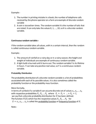
Random variable:- A variable whosevalueis determined by the outcome of
randomexperiment is called randomvariable.
The value of the randomvariable will vary fromtrial to trial as the experiment is
repeated. Random variable is also called chance variableor stochastic variable.
There are two types of random variable - discrete and continuous.
A random variable has either an associated probability distribution (discrete random
variable) or probability density function (continuous random variable).
Discrete randomvariable:-
If the random variable takes on the integer values such as 0,1,2, … then it is called
discrete random variable.

6. Example:-
1. The number in printing mistake in a book, the number of telephone calls
received by the phone operator on a farm areexample of discrete random
variable
2. A coin is tossed ten times. The randomvariable X is the number of tails that
are noted. X can only take the values 0, 1, ..., 10, so X is a discrete random
variable.
Continuous random variable:-
If the randomvariable takes all values, with in a certain interval, then the random
is called continuous randomvariable.
Example:-
1. The amount of rainfall on a rainy day or in a rainy season, the height and
weight of individuals are example of continuous randomvariable.
2. A light bulb is burned until it burns out. The randomvariable Y is its lifetime
in hours. Y can take any positive real value, so Y is a continuous random
variable.
Probability Distribution
The probability distribution of a discrete randomvariable is a list of probabilities
associated with each of its possiblevalues. Itis also sometimes called the
probability function or the probability mass function.
More formally,
In terms of symbols if a variableX can assumediscrete set of values 𝑥1, 𝑥2, … 𝑥 𝑘
with respective probabilities 𝑃1, 𝑃2, … 𝑃𝑘 where 𝑃1 + 𝑃2 + …+ 𝑃𝑘 = 1,
we say that a discrete probability distribution for 𝑋 has been defined.
The function 𝑃(𝑋) which has the respectivevalues 𝑃1 , 𝑃2 , … 𝑃𝑘 for
𝑋 = 𝑥1, 𝑥2,… 𝑥 𝑘 is called the probability function or frequency function of 𝑋.
Note:-

7. a. 0 ≤ 𝑃(𝑥𝑖) ≤ 1
b. ∑𝑃( 𝑥𝑖) = 1
ExpectedValue:-
The expected value (or population mean) of a randomvariable indicates its
averageor central value. Itis a useful summary value (a number) of the variable's
distribution.
Stating the expected value gives a general impression of the behavior of some
randomvariable without giving full details of its probability distribution (if it is
discrete) or its probability density function (if it is continuous).
Two randomvariables with the same expected value can havevery different
distributions. There are other usefuldescriptivemeasures which affect the shape
of the distribution, for example variance.
The expected value of a randomvariable X is symbolized by E(X) or µ.
If 𝑋 is a discrete randomvariable with possible values 𝑎1, 𝑎2,… 𝑎 𝑘 with respective
probabilities 𝑃1 , 𝑃2 ,… 𝑃𝑘 where 𝑃1 + 𝑃2 + …+ 𝑃𝑘 =1the mathematical
expectation of 𝑋 is defined as:
𝜇 = 𝐸( 𝑋) = ∑ 𝑋(𝑎𝑖)𝑃(𝑎𝑖)
Where the elements are summed over all values of the randomvariable X.
If X is a continuous randomvariablewith probability density function f(x), then
the expected value of X is defined by:
𝜇 = 𝐸( 𝑋) = ∫ 𝑥𝑓( 𝑥) 𝑑𝑥
Example

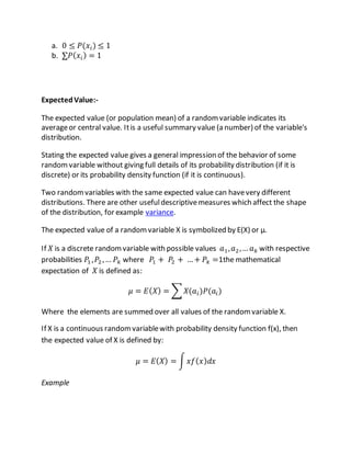
8. Discrete case: When a die is thrown, each of the possiblefaces 1, 2, 3, 4, 5, 6 (the
𝑥𝑖's) has a probability of 1/6 (the 𝑃(𝑥𝑖)'s) of showing. Theexpected value of the
face showing is therefore:
µ = 𝐸( 𝑋) = (1 ×
1
6
) + (2 ×
1
6
) + (3 ×
1
6
) + (4 ×
1
6
)
+ (5 ×
1
6
) + (6 ×
1
6
) = 3.5
Notice that, in this case, 𝐸(𝑋) is 3.5, which is not a possiblevalue of 𝑋.
Variance of 𝑋 = 𝑉𝑎𝑟( 𝑋) = 𝜎2
= 𝐸( 𝑋2) − [ 𝐸(𝑋)]2
Standard Deviationof 𝑿 = 𝝈
Example:-
Find expectation of the number of points when a fair die is rolled.
Solution:-
Let 𝑋 be the randomvariable showing number of points. Then 𝑋 = 1,2,3,4,5,6
𝑎𝑖 𝑃(𝑋 = 𝑎𝑖) = 𝑃(𝑎𝑖) Product
1
1
6
1
6
2
1
6
2
6
3
1
6
3
6
4
1
6
4
6
5
1
6
5
6
6
1
6
6
6
________________
𝐸( 𝑋) =
21
6
=
7
2
Expectation =
7
2
.

9. Normal Distribution
In probability theory, the normal (or Gaussian) distribution is a very commonly
occurring continuous probability distribution .
Strictly, a Normalrandomvariable should be capable of assuming any valueon
the real line, though this requirement is often waived in practice. For example,
height at a given age for a given gender in a given racial group is adequately
described by a Normal randomvariableeven though heights mustbe positive.
A continuous randomvariable X is said to follow a Normal distribution with
parameters µ and 𝜎 if it has probability density function
𝑓( 𝑥) = 𝑓(𝑥, 𝜇, 𝜎 ) =
1
𝜎√2𝜋
𝑒
( 𝑥−𝜇)2
2𝜎2
−∞ ≤ 𝑥 ≤ ∞, 𝜎 > 0,−∞ < 𝜇 < ∞
In such situation we write 𝑋~𝑁( 𝜇, 𝜎2)
The distribution involves two parameters 𝜇 and 𝜎2 .
Properties:-
a) Distribution is symmetrical.
b) 𝑀𝑒𝑎𝑛 = 𝜇, 𝑉𝑎𝑟𝑖𝑎𝑛𝑐𝑒 = 𝜎2 .

10. c) Mean , median and mode coincide.
d) 𝑓(𝑥) ≥ 0 for all 𝑥.
e) ∫ 𝑥𝑓( 𝑥) 𝑑𝑥
∞
−∞
= 1 i.e. Total area under the curve 𝑦 = 𝑓(𝑥) bounded by the
axix of 𝑥 is 1.
𝑁𝑜𝑡𝑒: −
a) Curvey-f(x), called normal curveis a bell shaped curve.
b) Itis symmetric about 𝑥 = 𝜇.
c) The two tails on the left and right sides of the mean extend to infinity.
d) Put 𝑧 =
𝑥−𝜇
𝜎
. Then 𝑍 is called a standard normalvariable and its
probability density function is given by 𝑃( 𝑧) =
1
√2𝜋
𝑒
−𝑧2
2 ,−∞ ≤ 𝑧 ≤ ∞.
e) Mean of the standard Normaldistributions is 0 and varianceis 1. Write
𝑍~𝑁(0,1)
The simplest case of a normaldistribution is known as the “standard
normaldistribution”.
Areaunder the standard normal curve:-
a) 𝐵𝑒𝑡𝑤𝑒𝑒𝑛 𝑧 = −1 𝑎𝑛𝑑 𝑧 = 1 𝑖𝑠 0.6827(Since total area under the standard
normal curveis 1)
𝑖. 𝑒. 𝑃(−1 < 𝑧 < 1) = 0.6827
b) 𝐵𝑒𝑡𝑤𝑒𝑒𝑛 𝑧 = −2 𝑎𝑛𝑑 𝑧 = 2 𝑖𝑠 0.9595
𝑖. 𝑒. 𝑃(−2 < 𝑧 < 2) = 0.9595
c) 𝐵𝑒𝑡𝑤𝑒𝑒𝑛 𝑧 = −3 𝑎𝑛𝑑 𝑧 = 3 𝑖𝑠 0.9973
𝑖. 𝑒. 𝑃(−3 < 𝑧 > 3) = 0.9973
In other words,

11. EXAMPLE: If a randomvariable has the normaldistribution with μ = 82.0 and σ=
4.8, Find the probabilities that it will take on a value
(a) less than 89.2
(b) greater than 78.4
(c) between 83.2 and 88.0
(d) between 73.6 and 90.4
Solution:
(a) We have

12. z =
89.2− 82
4.8
= 1.5
therefore the probability is 0.4332 + 0.5 = 0.9332.
(b) We have
𝑧 =
78.4− 82
4.8
= −0.75
therefore the probability is 0.2734 + 0.5 = 0.7734 .
(c) We have
𝑧1 =
83.2−82
4.8
= 0.25and 𝑧2 =
88−82
4.8
= 1.25
therefore the probability is 0.3944− 0.0987 = 0.2957.
(d) We have 𝑧1 =
73.6−82
4.8
= −1.75and 𝑧2 =
90.4−82
4.8
= 1.75
𝑡hereforethe probability is 0.4599 + 0.4599 = 0.9198.
Applications of the Normal Distribution
EXAMPLE: Intelligence quotients (IQs) measured on the Stanford Revision of the
Binet-Simon Intelligence Scale are normally distributed with a mean of 100 and a
standard deviation of 16.
Determine the percentage of people who haveIQs between 115 and 140.
Solution: We have 𝑧1 =
115−100
16
= 0.9375 and 𝑧2 =
140−100
16
= 2.5
therefore the probability is 0.4938− 0.3264 = 0.1674.
Itfollows that 16.74% of allpeople have IQs between 115 and 140. Equivalently,
the probability is 0.1674 thata randomly selected person will havean IQ between
115 and 140.
Many distribution tend to a normaldistribution in the limit.
When a variable is not normal, it can be made normal using using suitable
transformation.
When the sample size is large distrubution of simple mean, simple variance etc.
approach normality. Thus distribution forms a basis for test of significance.
Normal distribution is also called distribution of errors.