Download to read offline


![%Read in an image. Because the image is a truecolor image, the
example converts it to grayscale.
RGB = imread('saturn.png');
I = rgb2gray(RGB);
%The example then add Gaussian noise to the image and then
displays the image.
J = imnoise(I,'gaussian',0,0.025);
imshow(J)
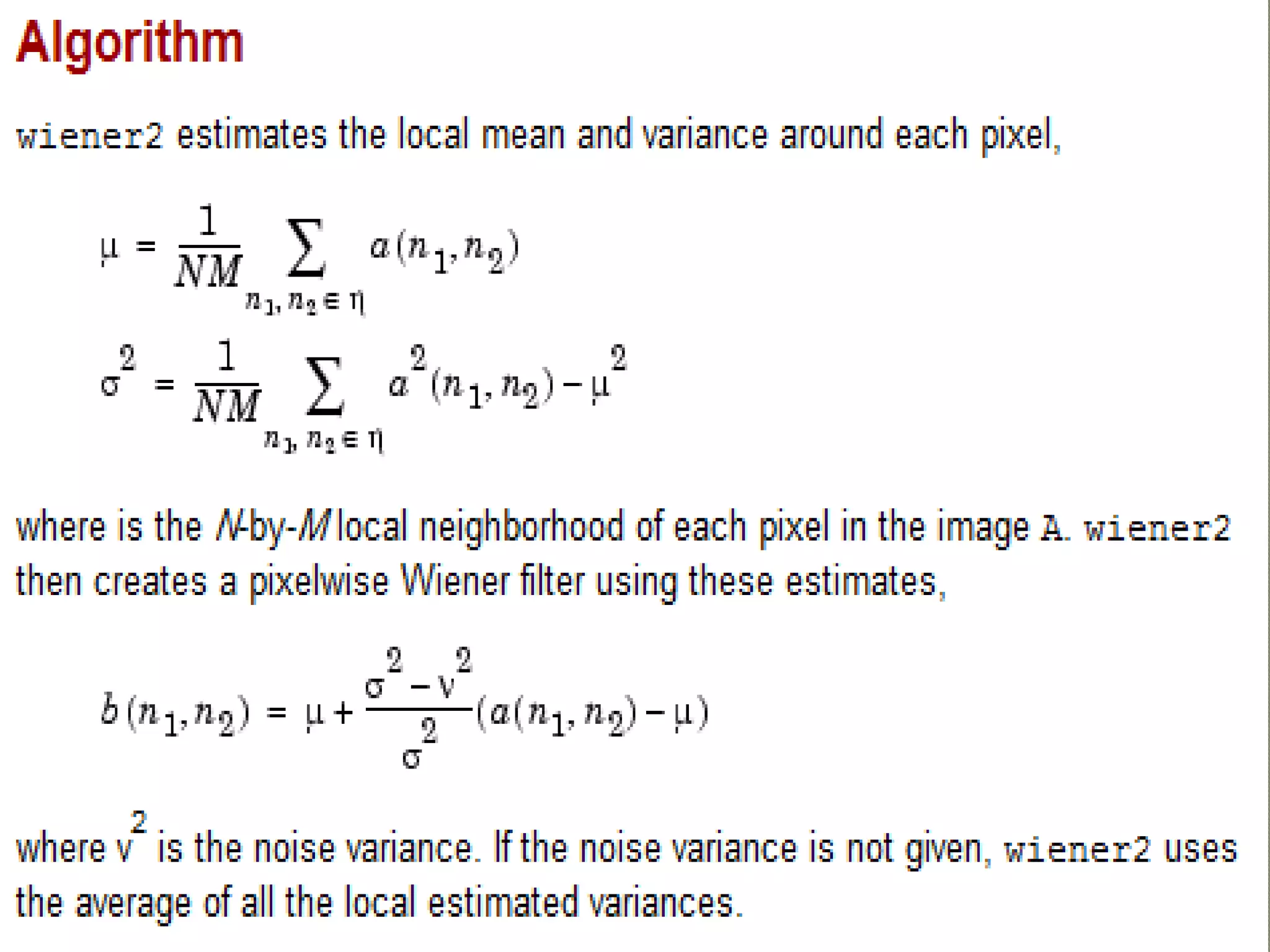
%Remove the noise, using the wiener2 function. Again, the figure only
shows a portion of the image
K = wiener2(J,[5 5]);
figure, imshow(K)](https://image.slidesharecdn.com/photometriccalibrationnew-150517104215-lva1-app6891/75/Photometric-calibration-16-2048.jpg)


![img=imread('v2.jpg');
av=mean(img(:));
[m,n]=size(img)
subplot(1,2,1)
imshow(img)
for i=1:m
for j=1:n
if (av-img(i,j))<(av/2)
img(i,j)=img(i,j)+(av/2);
end
end
end
subplot(1,2,2)
imshow(img)](https://image.slidesharecdn.com/photometriccalibrationnew-150517104215-lva1-app6891/75/Photometric-calibration-24-2048.jpg)

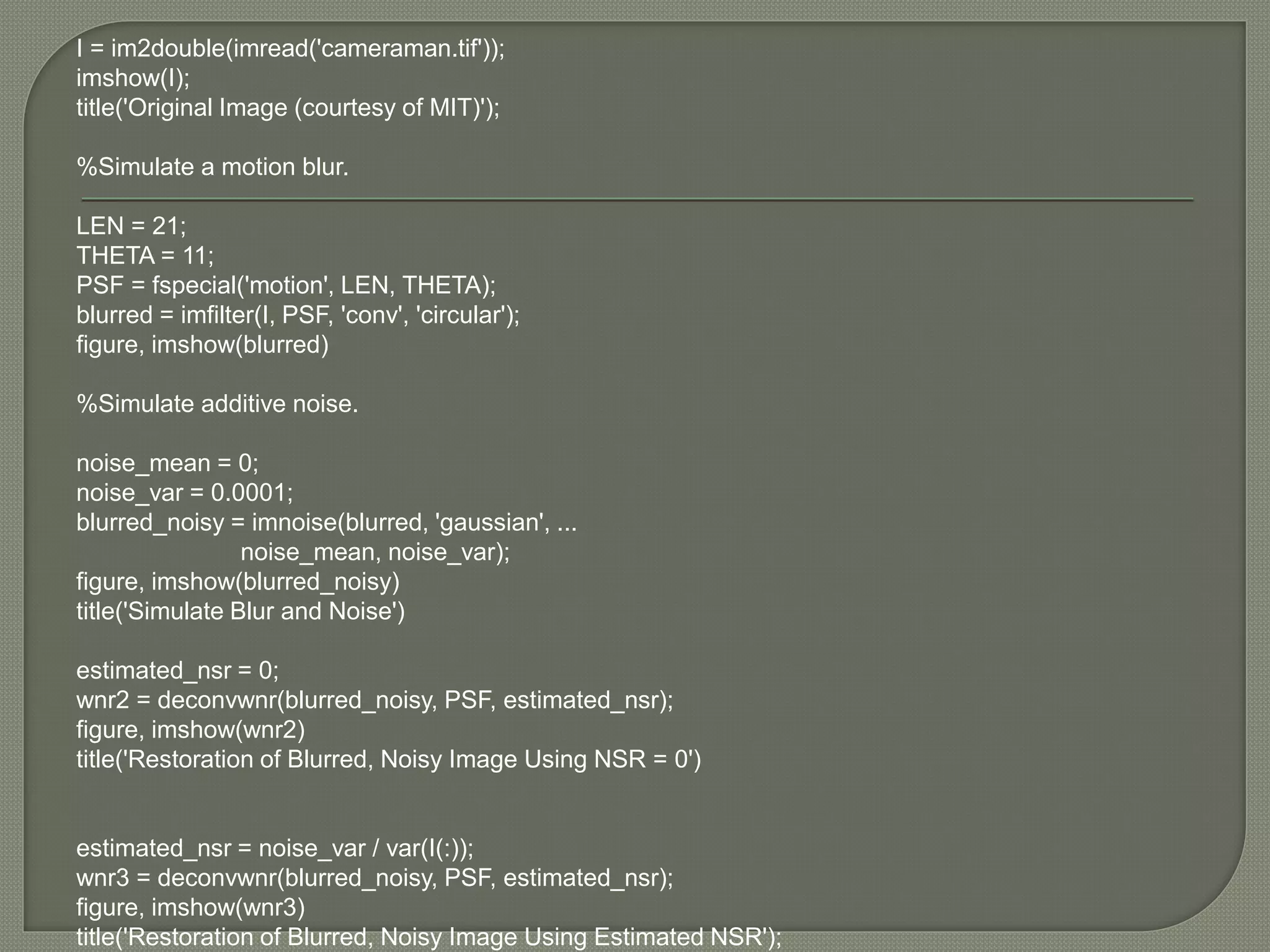
![I = imread('peppers.png');
I = I(60+[1:256],222+[1:256],:); % crop the image
figure; imshow(I); title('Original Image');
LEN = 31;
THETA = 11;
PSF = fspecial('motion',LEN,THETA); % create PSF
Blurred = imfilter(I,PSF,'circular','conv');
figure; imshow(Blurred); title('Blurred Image');
% Load image
I = im2double(Blurred);
figure(4); imshow(I); title('Source image');
%PSF
PSF = fspecial('motion', 14, 0);
noise_mean = 0;
noise_var = 0.0001;
estimated_nsr = noise_var / var(I(:));
I = edgetaper(I, PSF);
figure(5); imshow(deconvwnr(I, PSF, estimated_nsr)); title('Result')](https://image.slidesharecdn.com/photometriccalibrationnew-150517104215-lva1-app6891/75/Photometric-calibration-27-2048.jpg)

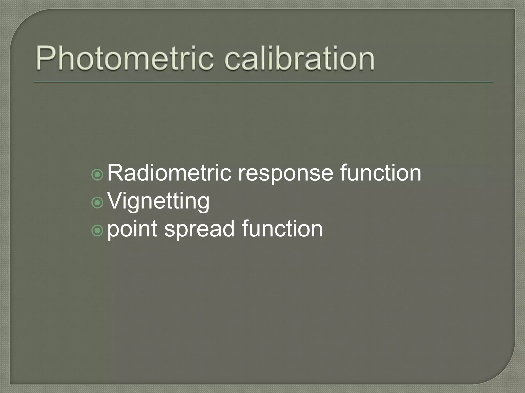
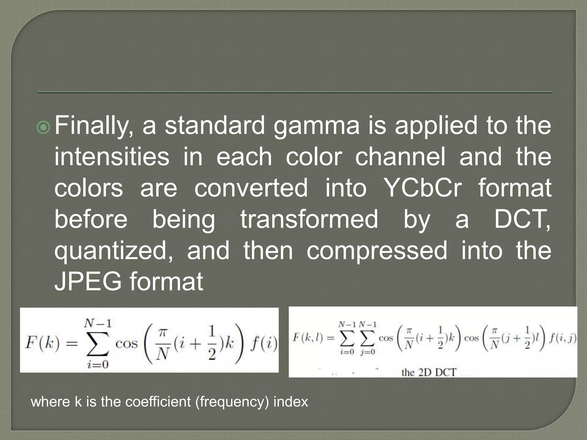
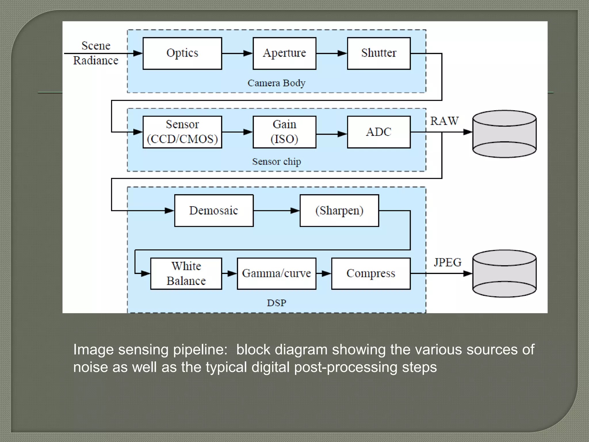
The document discusses various factors that affect the mapping of light intensity arriving at a camera lens to digital pixel values stored in an image file. It describes the radiometric response function, vignetting, and point spread function, which characterize how light is mapped and degraded by the camera imaging system. Sources of noise during image sensing and processing steps are also outlined. Methods to model and remove vignetting effects as well as deconvolve blur and noise in images using estimated point spread functions and noise levels are presented.