Downloaded 74 times


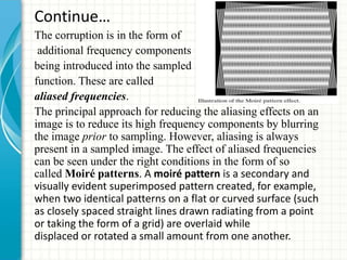
![Continue…
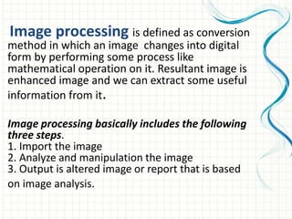
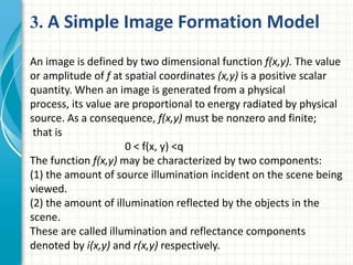
The two function combine as product to form f(x,y):
f(x,y)=i(x,y) r(x,y)
Where 0 < i(x,y)< ∞
and 0 <r(x,y)< 1
r(x,y)=0 means total absorption
r(x,y)=1 means total reflectance
We call the intensity of a monochrome image at any
coordinates (x,y) the gray level (l) of the image at that point.
That is l=f(x,y).
The interval of l ranges from [0,L-1]. Where l=0 indicates
black and l=1 indicates white. All the intermediate values are
shades of gray varying from black to white.](https://image.slidesharecdn.com/advanceimageprocessing-170913181745/85/Advance-image-processing-14-320.jpg)
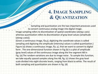
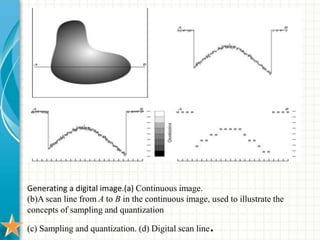


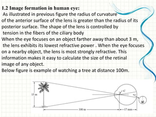
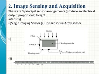
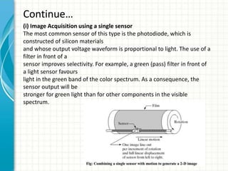
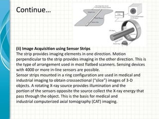
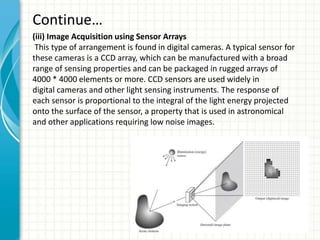
The document discusses key concepts in image processing including image sensing, acquisition, formation, sampling, quantization, and digital representation. It describes how the human eye forms images and contains photoreceptor cells. There are three main types of image sensors: single, line, and array. Sampling converts a continuous image to digital by selecting pixel values at regular intervals while quantization assigns discrete brightness levels. Together they allow images to be represented digitally as matrices of pixel values.


![Dimension reduction techniques[Feature Selection]](https://cdn.slidesharecdn.com/ss_thumbnails/dimensionreductiontechnibyaakankshajain-210625102243-thumbnail.jpg?width=640&height=640&fit=bounds)


![제 23회 보아즈(BOAZ) 빅데이터 컨퍼런스 - [MBOAX] : ABSA를 활용한 소비자 반응 분석 기반 운영 효율화 대시보드 설계](https://cdn.slidesharecdn.com/ss_thumbnails/3-1boaz23rdconferencemboax-260203102709-9d519923-thumbnail.jpg?width=640&height=640&fit=bounds)


