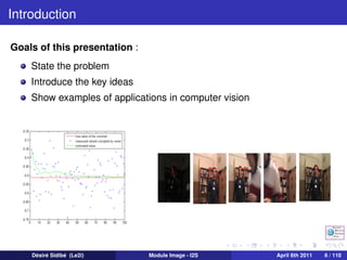
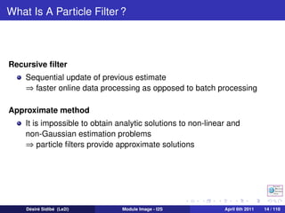
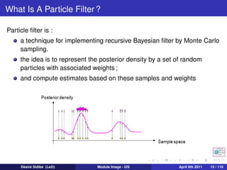
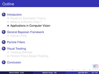
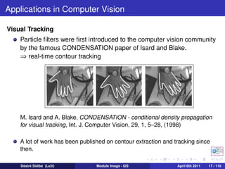
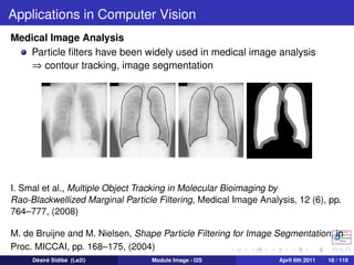
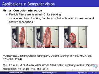
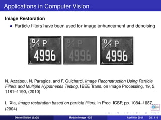
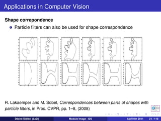
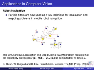
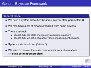
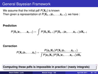
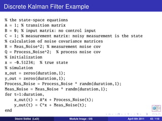
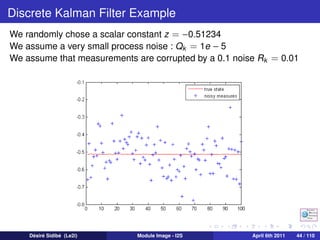
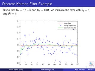
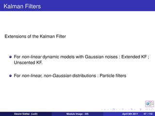
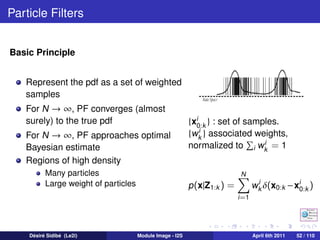
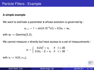
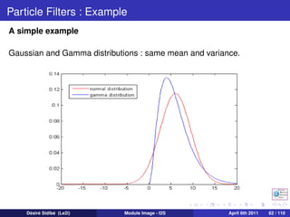
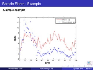
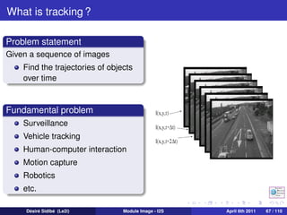
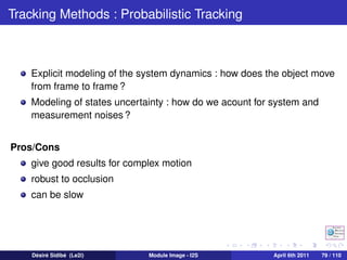
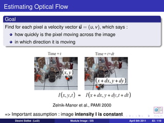
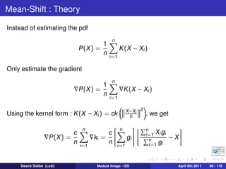
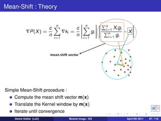
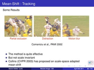
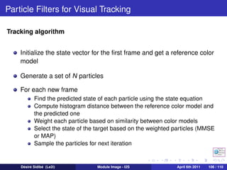
The document discusses particle filters and their applications in computer vision. It begins with an introduction to particle filters, which use a set of randomly chosen weighted samples to approximate a probability density function. Particle filters can be used for state estimation problems in nonlinear and non-Gaussian systems. The document then discusses several applications of particle filters in computer vision, including visual tracking, medical image analysis, human-computer interaction, image restoration, and robot navigation. Finally, it provides an outline of topics to be covered, including the general Bayesian framework, particle filtering methods, visual tracking techniques, and conclusions.


![Discrete Kalman Filters
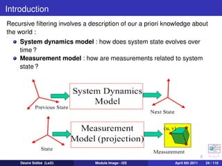
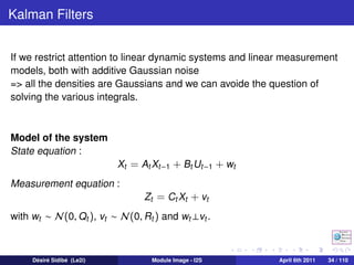
Importance of Gaussian distribution
Since the system is linear and the distributions are Gaussian, we need
only to know
the conditional mean Xk = E[Xk |Z1:k , U0:k −1 ]
the conditional covariance Pk = Cov (Xk , Xk |Z1:k , U0:k −1 )
Recursivity
Assume that we know P (xk |Z1:k , U0:k −1 ) at some time k
1 Prediction : what can we say about xk +1 before we get the
measurement Zk +1 ?
P (xk +1 |Z1:k , U0:k )
2 Correction : how can we improve our knowledge of xk +1 given the
actual measurement zk +1 ?
P (xk +1 |Z1:k +1 , U0:k )
Désiré Sidibé (Le2i) Module Image - I2S April 6th 2011 35 / 110](https://image.slidesharecdn.com/sidibemoduleimage2011-120307023650-phpapp02/85/Particle-Filters-and-Applications-in-Computer-Vision-35-320.jpg)
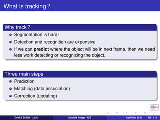
![Discrete Kalman Filters
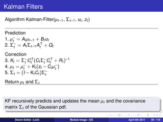
ˆ
Assume we know xk and Pk .
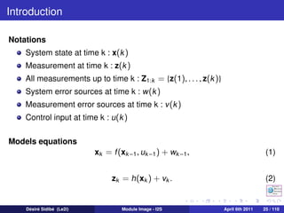
Prediction step
From the state equation :
ˆ−
xk +1 = E[xk +1 |Z1:k , U0:k ]
= Ak xk + Bk uk .
ˆ
From the prior estimate error covariance
− ˆ− ˆ−
Pk +1 = E[(xk +1 − xk +1 )(xk +1 − xk +1 )T ]
= Ak Pk Ak + Qk .
T
Désiré Sidibé (Le2i) Module Image - I2S April 6th 2011 36 / 110](https://image.slidesharecdn.com/sidibemoduleimage2011-120307023650-phpapp02/85/Particle-Filters-and-Applications-in-Computer-Vision-36-320.jpg)
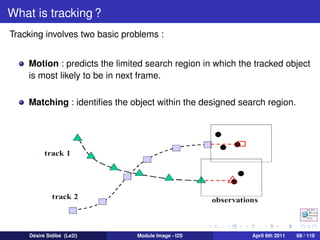
![Discrete Kalman Filters
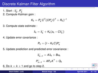
Correction step
Use the measurement equation to make a prediction of the
observation
zk +1 = Ck +1 xk +1 .
− ˆ−
Given, the actual observation zk +1 , correct the state prediction
ˆ ˆ− −
xk +1 = xk +1 + Kk +1 (zk +1 − zk +1 ).
−
(zk +1 − zk +1 ) is called the measurement innovation or the residual.
Kk +1 is called the Kalman gain and is chosen in order to minimize the
posterior MMSE Pk +1 = E[(xk +1 − xk +1 )(xk +1 − xk +1 )T ].
ˆ ˆ
Désiré Sidibé (Le2i) Module Image - I2S April 6th 2011 37 / 110](https://image.slidesharecdn.com/sidibemoduleimage2011-120307023650-phpapp02/85/Particle-Filters-and-Applications-in-Computer-Vision-37-320.jpg)
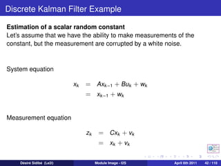
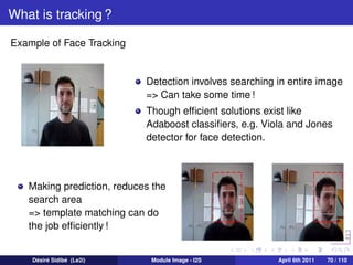
![Discrete Kalman Filters
Optimal Kalman Gain
The a posteriori error covariance matrix is
Pk +1 = E[(xk +1 − xk +1 )(xk +1 − xk +1 )T ],
ˆ ˆ
which after a few calculations gives
Pk +1 = (I − Kk +1 Ck +1 )Pk +1 (I − Kk +1 Ck +1 )T + Kk +1 Rk +1 Kk +1 .
− T
Taking the trace of Pk +1 and setting its derivative w.r.t. Kk +1 equals to
zero, we obtain the optimal Kalman gain
Kk +1 = Pk +1 Ck +1 [Ck +1 Pk +1 Ck +1 + Rk +1 ]−1 .
− T − T
The posterior covariance matrix can then be simplified as
Pk +1 = (I − Kk +1 Ck +1 )Pk +1 .
−
Désiré Sidibé (Le2i) Module Image - I2S April 6th 2011 38 / 110](https://image.slidesharecdn.com/sidibemoduleimage2011-120307023650-phpapp02/85/Particle-Filters-and-Applications-in-Computer-Vision-38-320.jpg)
![Discrete Kalman Filters
In most of our applications, the matrices Ak , Bk and Ck do not vary over
time. So, the Kalman filter equations are simplified as :
Prediction step
ˆ− ˆ
xk +1 = A xk + Buk
−
Pk +1 = APk A T + Qk
Correction step
Kk +1 = Pk +1 C T [CPk +1 C T + Rk +1 ]−1
− −
ˆ ˆ− ˆ−
xk +1 = xk +1 + Kk +1 (zk +1 − C xk +1 )
−
Pk +1 = (I − Kk +1 C )Pk +1
Désiré Sidibé (Le2i) Module Image - I2S April 6th 2011 40 / 110](https://image.slidesharecdn.com/sidibemoduleimage2011-120307023650-phpapp02/85/Particle-Filters-and-Applications-in-Computer-Vision-40-320.jpg)
![Discrete Kalman Filter Code
function [x_out]=discrete_kalman_filter(y, u, x0, P0, A,B,C,Q,R)
T = size(y, 1); %number of observations
[n,m] = size(P0); I = eye(n,m); % form identity matrix
xhat = x0; P = P0; %initialization
x_out = [];
for k=1:T,
% compute Kalman Gain
K = P*C’* inv(C*P*C’ + R);
% estimate state
innovation = y(k) - C*xhat; % innovation vector
xhat = xhat + K*innovation;
x_out = [x_out; xhat’];
% update covariance matrice
P = (I - K*C)*P;
% predict next state and covariance
xhat = A*xhat + B*u;
P = A*P*A’ + Q;
end
Désiré Sidibé (Le2i) Module Image - I2S April 6th 2011 45 / 110](https://image.slidesharecdn.com/sidibemoduleimage2011-120307023650-phpapp02/85/Particle-Filters-and-Applications-in-Computer-Vision-45-320.jpg)
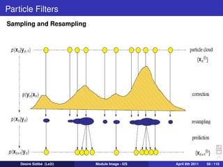
![Particle Filters
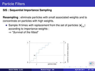
SIS : Sequential Importance Sampling
Pseudo-code
A 1 : SIS Particle Filter
[{xik , wk }N 1 ] = SIS [{xik −1 , wk −1 }N 1 , zk ]
i
i=
i
i=
For i = 1 : N
Draw xik ∼ q(xk |xik −1 , zk )
Update weights according to
i i
p (zk |xik )p (xik |xik −1 )
wk ∝ wk −1
q(xik |xik −1 , zk )
End For
N i
Normalize weights to i =1 wk = 1
Désiré Sidibé (Le2i) Module Image - I2S April 6th 2011 55 / 110](https://image.slidesharecdn.com/sidibemoduleimage2011-120307023650-phpapp02/85/Particle-Filters-and-Applications-in-Computer-Vision-55-320.jpg)
![Particle Filters
Generic Particle Filter Pseudo-Code
A 2 : Generic Particle Filter
[{xik , wk }N 1 ] = PF [{xik −1 , wk −1 }N 1 , zk ]
i
i=
i
i=
FOR i = 1 : N
Draw xik ∼ q(xk |xik −1 , zk )
i i p (zk |xik )p (xik |xik −1 )
Update weights according to wk ∝ wk −1 q(xik |xik −1 ,zk )
END FOR
N i
Normalize weights to i =1 wk = 1
1
Calculate degeneracy measure : Neff = N i 2
i =1 (wk )
IF Neff < NT
Resample
END IF
Désiré Sidibé (Le2i) Module Image - I2S April 6th 2011 59 / 110](https://image.slidesharecdn.com/sidibemoduleimage2011-120307023650-phpapp02/85/Particle-Filters-and-Applications-in-Computer-Vision-59-320.jpg)
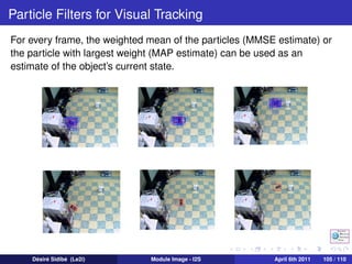
![Particle Filters
Estimation form particles
Any estimate of a function f (xk ) can be obtained from the discrete pdf
approximation :
N
1
E[f (xk )] = wk f (xik )
i
N
i =1
1 N
Mean : E[xk ] = N i =1 wk xik
i
MAP estimate : particle with largest weight
Robust mean : mean within window around MAP estimate
Désiré Sidibé (Le2i) Module Image - I2S April 6th 2011 60 / 110](https://image.slidesharecdn.com/sidibemoduleimage2011-120307023650-phpapp02/85/Particle-Filters-and-Applications-in-Computer-Vision-60-320.jpg)
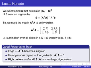
![Lucas Kanade
Local smoothness
u
Ix u + Iy v = −It =⇒ [Ix Iy ] = −It
v
If we assume constant velocity (u, v ) in small neighborhood
Ix1 Iy1 It1
Ix2 Iy2
u
It2
Ix3 Iy3
v
= −
It3
. . .
. . .
. . .
We get an over-determined system
Au = b
which we can solve using LLS (Linear Least Squares) method.
Désiré Sidibé (Le2i) Module Image - I2S April 6th 2011 86 / 110](https://image.slidesharecdn.com/sidibemoduleimage2011-120307023650-phpapp02/85/Particle-Filters-and-Applications-in-Computer-Vision-86-320.jpg)
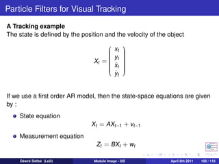
![Particle Filters for Visual Tracking
Since color is a distinctive and quite robust feature, each particle is
dscribed by the color distribution of its local image patch,
p (x) = {pu (x)}u=1,...,m given by :
Np 2
xi − x
pu (x) = C k( )δ[b (xi ) − u],
h
i =1
where C is a normalizer, δ is the Kronecker function, k is a kernel with
bandwith h, Np is the number of pixels in the region and b (xi ) is a
function that assigns one of the m-bins to a given color at location xi .
The kernel k is used to consider spatial information by lowering the
contribution of farther pixels.
Désiré Sidibé (Le2i) Module Image - I2S April 6th 2011 103 / 110](https://image.slidesharecdn.com/sidibemoduleimage2011-120307023650-phpapp02/85/Particle-Filters-and-Applications-in-Computer-Vision-103-320.jpg)
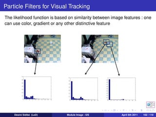
![Particle Filters for Visual Tracking
The similarity between two color distributions, p (xt ) and p ∗ (x0 ), can
be defined as the Bhattacharyya distance
m
1
2
ρ[p ∗ , p (xt )] = 1 − ∗
pu (x0 )pu (xt )
u=1
Each sample xit is assigned an importance weight which corresponds
to the likelihood that xit is the true location of the object. The weights
are given by the observation likelihood :
∗ ,p (xi )]2
wti = p (zt |xit ) ∝ e −λρ[p t .
Désiré Sidibé (Le2i) Module Image - I2S April 6th 2011 104 / 110](https://image.slidesharecdn.com/sidibemoduleimage2011-120307023650-phpapp02/85/Particle-Filters-and-Applications-in-Computer-Vision-104-320.jpg)
![[PR12] You Only Look Once (YOLO): Unified Real-Time Object Detection](https://cdn.slidesharecdn.com/ss_thumbnails/yolo-170616085751-thumbnail.jpg?width=640&height=640&fit=bounds)


![Sensor Fusion Study - Ch15. The Particle Filter [Seoyeon Stella Yang]](https://cdn.slidesharecdn.com/ss_thumbnails/particlefilter-200815094542-thumbnail.jpg?width=640&height=640&fit=bounds)