Strata 2013: Tutorial-- How to Create Predictive Models in R using Ensembles

How to Create Predictive Models in
R using Ensembles
Giovanni Seni, Ph.D.
Intuit
@IntuitInc

Giovanni_Seni@intuit.com
Santa Clara University
GSeni@scu.edu

Strata - Hadoop World, New York
October 28, 2013

Reference

© 2013 G.Seni

2013 Strata Conference + Hadoop World

2

Overview
•  Motivation, In a Nutshell & Timeline
•  Predictive Learning & Decision Trees
•  Ensemble Methods - Diversity & Importance Sampling
–  Bagging
–  Random Forest
–  Ada Boost
–  Gradient Boosting
–  Rule Ensembles

•  Summary

© 2013 G.Seni


3

Motivation

Volume 9 Issue 2

© 2013 G.Seni


4

Motivation (2)

“1′st Place Algorithm Description: … 4. Classification: Ensemble classification methods are used to combine
multiple classifiers. Two separate Random Forest ensembles are created based on the shadow index (one for the
shadow-covered area and one for the shadow-free area). The random forest “Out of Bag” error is used to
automatically evaluate features according to their impact, resulting in 45 features selected for the shadow-free and
55 for the shadow-covered part.”
© 2013 G.Seni


5

Motivation (3)
•  “What are the best of the best techniques at winning
Kaggle competitions?
–  Ensembles of Decisions Trees
–  Deep Learning

account for 90% of top 3 winners!”
Jeremy Howard, Chief Scientist of Kaggle
KDD 2013
⇒ Key common characteristics:
–  Resistance to overfitting
–  Universal approximations
© 2013 G.Seni


6

Ensemble Methods in a Nutshell
•  “Algorithmic” statistical procedure
•  Based on combining the fitted values from a number of
fitting attempts
•  Loosely related to:
–  Iterative procedures
–  Bootstrap procedures

•  Original idea: a “weak” procedure can be strengthened if
it can operate “by committee”
–  e.g., combining low-bias/high-variance procedures

•  Accompanied by interpretation methodology
© 2013 G.Seni


7

Timeline
•  CART (Breiman, Friedman, Stone, Olshen, 1983)
•  Bagging (Breiman, 1996)
–  Random Forest (Ho, 1995; Breiman 2001)

•  AdaBoost (Freund, Schapire, 1997)
•  Boosting – a statistical view (Friedman et. al., 2000)
–  Gradient Boosting (Friedman, 2001)
–  Stochastic Gradient Boosting (Friedman, 1999)

•  Importance Sampling Learning Ensembles (ISLE)
(Friedman, Popescu, 2003)
© 2013 G.Seni


8

Timeline (2)
•  Regularization – variance control techniques:
–  Lasso (Tibshirani, 1996)
–  LARS (Efron, 2004)
–  Elastic Net (Zou, Hastie, 2005)
–  GLMs via Coordinate Descent (Friedman, Hastie, Tibshirani, 2008)

•  Rule Ensembles (Friedman, Popescu, 2008)

© 2013 G.Seni


9

Overview
Ø  Predictive Learning & Decision Trees
•  Ensemble Methods
•  Summary

© 2013 G.Seni


10

Predictive Learning
Procedure Summary
N
N
•  Given "training" data D = { yi , xi1 , xi 2 ,, xin }1 = { yi , x i }1

–  D is a random sample from some unknown (joint) distribution


 
•  Build a functional model y = F ( x1 , x2 ,, xn ) = F ( x )
–  Offers adequate and interpretable description of how the inputs
affect the outputs
–  Parsimony is an important criterion: simpler models are preferred
for the sake of scientific insight into the x - y relationship

•  Need to specify: < model, score criterion, search strategy >
© 2013 G.Seni


11

Predictive Learning
Procedure Summary (2)
•  Model: underlying functional form sought from data


F (x) = F (x; a) ∈ ℱ

family of functions indexed by a

•  Score criterion: judges (lack of) quality of fitted model


–  Loss function L( y, F ): penalizes individual errors in prediction

–  Risk R(a) = E y ,x L( y, F (x; a)) : the expected loss over all predictions

•  Search Strategy: minimization procedure of score criterion
a* = arg min R(a)
a

© 2013 G.Seni


12

Predictive Learning
Procedure Summary (3)
•  “Surrogate” Score criterion:
N
–  Training data: { yi , x i }1 ~ p( x, y )

*
–  p ( x, y ) unknown ⇒ a unknown

⇒ Use approximation: Empirical Risk


1
•  R (a) =
N


∑ L( y, F (xi ; a))
N

i =1

•  If not N >> n ,

© 2013 G.Seni

⇒



a = arg min R(a)
a


R(a) >> R(a* )


13

Predictive Learning
Example
•  A simple data set
Attribute-1

Attribute-2

Class

( x1 )

( x2 )

1.0

2.0

blue

2.0

1.0

green

…

…

…

4.5

3.5

x2

?

(y)

•  What is the class of new point

x1

?

•  Many approaches… no method is universally better; try
several / use committee
© 2013 G.Seni


14

Predictive Learning
Example (2)
•  Ordinary Linear Regression (OLR)
x2

x1

n

–  Model: F(x) = a0 + ∑ a j x j
j=1

;


⎧
F (x) ≥ 0 ⎨
⎩else

⇒ Not flexible enough
© 2013 G.Seni


15

Decision Trees
Overview
x2
R2

x1 ≥ 5

R1

x2 ≥ 3

3

R4

x1 ≥ 2

R3
2

x1

5

M

ˆ
ˆ ˆ
•  Model: y = T (x ) = ∑ cm I R (x )
m =1

m

 M
{Rm }m=1 =

Sub-regions of input
variable space

where I R (x) = 1 if x ∈ R , 0 otherwise
© 2013 G.Seni


16

Decision Trees
Overview (2)
•  Score criterion:
–  Classification – "0-1 loss" ⇒ misclassification error (or surrogate)
N

M

ˆ
{ cˆm, Rm } = argmin
1

M
cm ,Rm 1

TM ={

}

∑I (y ≠ T
i

M

(x i ))

i=1

2

ˆ
ˆ
–  Regression – least squares – i.e., L( y , y ) = ( y − y )
M

ˆ ˆ
{ cm, Rm } = argmin
1

M

N

∑( y − T
i

TM ={cm ,Rm }1 i=1

M

(x i ))


R(TM )

2



•  Search: Find T = arg min T R(T )
–  i.e., find best regions Rm and constants cm
© 2013 G.Seni


17

Decision Trees
Overview (3)
•  Join optimization with respect to Rm and cm simultaneously is
very difficult
⇒ use a greedy iterative procedure
R0

R4

R1

R5 R6

R2

R3

•

•

j 1 , s1

R0
j 2 , s2

•

•

j 1 , s1

R0
j 2 , s2

R1

•

R0

•

R1

•
R3

•

j 1 , s1

•
R4

j 3 , s3

j 2 , s2

•

j 1 , s1

R0

•
R3

••

•

R4 R5
R7


j 4 , s4

R6

•
© 2013 G.Seni

j 3 , s3

R2

R1

R2

•

•
R8
18

Decision Trees
What is the “right” size of a model?
y

y

y

ο ο ο
ο
ο
ο ο

ο ο

ο ο ο

ο ο

ο

⇒

ο
ο

ο

c1

ο

ο ο

x

ο ο

ο ο

ο ο

ο ο ο

c2

ο

vs

ο
ο

c1 ο

c2

ο ο

ο

ο ο

ο
ο ο

ο ο

c3

ο
ο

ο

ο

x

x

•  Dilemma
–  If model (# of splits) is too small, then approximation is too crude
(bias) ⇒ increased errors
–  If model is too large, then it fits the training data too closely
(overfitting, increased variance) ⇒ increased errors
© 2013 G.Seni


19

Decision Trees
What is the “right” size of a model? (2)
High Bias

Low Bias

Low Variance

Prediction Error

High Variance

Test Sample

Training Sample
Low

M*

High

Model Complexity

–  Right sized tree, M * when test error is at a minimum
,
–  Error on the training is not a useful estimator!
•  If test set is not available, need alternative method
© 2013 G.Seni


20

Decision Trees
Pruning to obtain “right” size
•  Two strategies
–  Prepruning - stop growing a branch when information becomes
unreliable
•  #(Rm) – i.e., number of data points, too small
⇒ same bound everywhere in the tree
•  Next split not worthwhile
⇒ Not sufficient condition

–  Postpruning - take a fully-grown tree and discard unreliable parts
(i.e., not supported by test data)
•  C4.5: pessimistic pruning
•  CART: cost-complexity pruning
© 2013 G.Seni

(more statistically grounded)


21

Decision Trees

1.0

Hands-on Exercise
Start Rstudio

• 

0.8

• 

Navigate to directory:
example.1.LinearBoundary

Load and run “fitModel_CART.R”

• 

If curious, also see
“gen2DdataLinear.R”

• 

After boosting discussion, load and
run “fitModel_GBM.R

0.0

0.2

0.4

x2

Set working directory: use
setwd() or with GUI

• 

0.6

• 

0.0

0.2

0.4

0.6

0.8

1.0

x1

© 2013 G.Seni


22

Decision Trees
Key Features
•  Ability to deal with irrelevant inputs
–  i.e., automatic variable subset selection
–  Measure anything you can measure
–  Score provided for selected variables ("importance")

•  No data preprocessing needed
-  Naturally handle all types of variables
• 

numeric, binary, categorical

-  Invariant under monotone transformations: x j = g j (x j )
• 
• 
© 2013 G.Seni

Variable scales are irrelevant
Immune to bad x j −distributions (e.g., outliers)

23

Decision Trees
Key Features (2)
•  Computational scalability
–  Relatively fast: O(nN log N )

•  Missing value tolerant
-  Moderate loss of accuracy due to missing values
-  Handling via "surrogate" splits

•  "Off-the-shelf" procedure
-  Few tunable parameters

•  Interpretable model representation
-  Binary tree graphic
© 2013 G.Seni


24

Decision Trees
Limitations
•  Discontinuous piecewise constant model
F (x)

x

–  In order to have many splits you need to have a lot of data
•  In high-dimensions, you often run out of data after a few splits

–  Also note error is bigger near region boundaries
© 2013 G.Seni


25

Decision Trees
Limitations (2)
•  Not good for low interaction F * (x )
n

*

–  e.g., F (x ) = ao + ∑ a j x j is worst function for trees
j =1

n

= ∑ f j* (x j )

(no interaction, additive)

j =1

–  In order for xl to enter model, must split on it
•  Path from root to node is a product of indicators

•  Not good for F * (x ) that has dependence on many variables
-  Each split reduces training data for subsequent splits (data
fragmentation)

© 2013 G.Seni


26

Decision Trees
Limitations (3)
•  High variance caused by greedy search strategy (local optima)
–  Errors in upper splits are propagated down to affect all splits
below it
⇒ Small changes in data (sampling fluctuations) can cause
big changes in tree
- Very deep trees might be questionable
- Pruning is important

•  What to do next?
–  Live with problems
–  Use other methods (when possible)
–  Fix-up trees: use ensembles
© 2013 G.Seni


27

Overview
•  In a Nutshell & Timeline
Ø  Ensemble Methods
–  In a Nutshell, Diversity & Importance Sampling
–  Generic Ensemble Generation
–  Bagging, RF, AdaBoost, Boosting, Rule Ensembles

•  Summary

© 2013 G.Seni


28

Ensemble Methods
In a Nutshell
M

•  Model: F (x) = c0 + ∑m=1 cmTm (x)
M
–  { m (x)}1 : “basis” functions (or “base learners”)
T

–  i.e., linear model in a (very) high dimensional space of derived
variables

•  Learner characterization:

Tm (x) = T (x; p m )

–  p m : a specific set of joint parameter values – e.g., split definitions
at internal nodes and predictions at terminal nodes
–  {T (x; p)}p∈P : function class – i.e., set of all base learners of specified
family
© 2013 G.Seni


29

Ensemble Methods
In a Nutshell (2)
•  Learning: two-step process; approximate solution to
N
M
  M
{cm , p m }o = arg min ∑ L yi , c0 + ∑ cmT (x;p m )
M
{cm , p m }o i=1

(

m=1

)

M
–  Step 1: Choose points {p m }1

M
•  i.e., select {Tm (x)}1 ⊂ {T (x; p)}p∈P

M
–  Step 2: Determine weights {cm }0

•  e.g., via regularized LR

© 2013 G.Seni


30

Ensemble Methods
Importance Sampling (Friedman, 2003)
•  How to judiciously choose the “basis” functions (i.e., {pm }1M )?
M
•  Goal: find “good” {pm }1 so that

M
M
F (x;{p m }1 , {cm }1 ) ≅ F * (x )

•  Connection with numerical integration:
– 

∫

Ρ

M

I (p) ∂p ≈ ∑m =1 w m I (p m )

vs.

© 2013 G.Seni


Accuracy improves
when we choose more
points from this
region…

31

Importance Sampling
Numerical Integration via Monte Carlo Methods
M
•  r (p) = sampling pdf of p ∈ P -- i.e, {p m ~ r (p)}1

–  Simple approach: r (p m ) iid -- i.e., uniform
–  In our problem: inversely related to p m’s “risk”
•  i.e., T (x; p m ) has high error ⇒ lack of relevance of p m ⇒ low r (pm )

•  “Quasi” Monte Carlo:
–  with/out knowledge of the other points that will be used
•  i.e., single point vs. group importance

–  Sequential approximation: p’s relevance judged in the context of
the (fixed) previously selected points
© 2013 G.Seni


32

Ensemble Methods
Importance Sampling – Characterization of
•  Let p∗ = arg minp Risk(p)

Narrow r (p)

Broad r (p)

M

T
•  Ensemble { (x; p m )}1 of “strong” base
learners - i.e., all with Risk (p m ) ≈ Risk (p∗ )

•  Diverse ensemble - i.e., predictions are
not highly correlated with each other

•  T (x; p m ) yield similar highly correlated
’s
predictions ⇒ unexceptional performance

•  However, many “weak” base learners - i.e.,
Risk (p m ) >> Risk (p ∗ ) ⇒ poor performance

© 2013 G.Seni


33

Ensemble Methods
Approximate Process of Drawing from
•  Heuristic sampling strategy: sampling around p by iteratively
applying small perturbations to existing problem structure
∗

–  Generating ensemble members Tm (x) = T (x; p m )

For m = 1 to M {
pm = PERTURBm { minp Ε xy L( y, T (x; p) )}
arg
}
⋅
–  PERTURB {} is a (random) modification of any of

•  Data distribution - e.g., by re-weighting the observations
•  Loss function - e.g., by modifying its argument
•  Search algorithm (used to find minp)


–  Width of r (p ) is controlled by degree of perturbation
© 2013 G.Seni


34

Generic Ensemble Generation
Step 1: Choose Base Learners p!

!
! !

•  Forward Stagewise Fitting Procedure:
𝐹0 (x) = 0
For 𝑚 = 1 to 𝑀 {

//
Fit
a
single
base
learner

p

Modification of
data distribution

𝑚

= argmin .
p

𝐿0𝑦 𝑖 , 𝐹 𝑚 −1 + 𝑇(x 𝑖 ; p)8

𝑖∈𝑆 𝑚 ( 𝜂 )

//
Update
additive
expansion

𝑇 𝑚 ( 𝑥 ) = 𝑇0x; p 𝒎 8

𝐹 𝑚 (x) = 𝐹 𝑚 −1 (x) + 𝜐 ∙ 𝑇 𝑚 (x)
}
write { 𝑇 𝑚 (x)}1𝑀

–  Algorithm control: L, η , υ

Modification of loss function
(“sequential” approximation)

•  Sm (η ) : random sub-sample of size η ≤ N ⇒ impacts ensemble "diversity"
m −1

•  Fm−1 (x) = υ ⋅ ∑k =1Tk (x) : “memory” function (0 ≤ υ ≤ 1 )
© 2013 G.Seni


35

Generic Ensemble Generation
Step 2: Choose Coefficients c!

!
!!

M
M
•  Given {Tm (x)}m=1 = {T (x; pm )}m=1 , coefficients can be obtained by a

regularized linear regression
N
M
⎛
⎞

{cm } = arg min ∑ L⎜ yi , c0 + ∑ cmTm (xi ) ⎟ + λ ⋅ P(c )
{cm }
i =1 ⎝
m =1
⎠

–  Regularization here helps reduce bias (in addition to variance) of the
model
–  New iterative fast algorithms for various loss/penalty combinations
•  “GLMs via Coordinate Descent” (2008)

© 2013 G.Seni


36

Bagging (Breiman, 1996)
•  Bagging = Bootstrap Aggregation
ˆ
•  L(y, y) : as available for single tree

F0 (x) = 0
For m = 1 to M {

•  υ = 0 ⇒ no memory

p m = arg min
p

•  η = N / 2

i

m −1

i∈S m ( )

( x i ) + T ( x i ; p ))

Tm (x) = T (x; p m )

•  Tm (x) ⇒ are large un-pruned
trees

∑ηL(y , F

Fm (x) = Fm −1 (x) + υ ⋅ Tm (x)
υ
}

•  co = 0, {cm = 1 / M }1M

M

i.e., not fit to the data (avg)

write {Tm (x)}1

–  i.e., perturbation of the data distribution only
–  Potential improvements?
–  R package: ipred
© 2013 G.Seni


37

Bagging
Hands-on Exercise

1.0

• 

example.2.EllipticalBoundary

0.0

Load and run
–  fitModel_Bagging_by_hand.R

-0.5

–  fitModel_CART.R (optional)
• 

If curious, also see
gen2DdataNonLinear.R

-1.0

x2

Set working directory: use setwd()
or with GUI

• 

0.5

• 

• 

After class, load and run
fitModel_Bagging.R

-2

-1

0

1

2

x1

© 2013 G.Seni


38

Bagging
Why it helps?

ˆ
•  Under L( y, y) = ( y − y) 2, averaging reduces variance and leaves
bias unchanged

•  Consider “idealized” bagging (aggregate)


estimator: f (x) = Ε f Z (x)



–  f Z fit to bootstrap data set Z = {yi , xi }1N
–  Z is sampled from actual population distribution (not training data)




–  We can write: Ε[Y − f Z (x)] = Ε[Y − f (x) + f (x) − f Z (x)]
2

2


2
= Ε Y − f ( x) + Ε f Z ( x) − f ( x)

[
]
≥ Ε[Y − f (x)]

[

]

2

2

⇒  true population aggregation never increases mean squared error!
⇒  Bagging will often decrease MSE…
© 2013 G.Seni


39

Random Forest (Ho, 1995; Breiman, 2001)
•  Random Forest = Bagging + algorithm randomizing
–  Subset splitting
As each tree is constructed…
•  Draw a random sample of predictors before each node is split

ns = ⎣log 2 (n) + 1⎦
•  Find best split as usual but selecting only from subset of predictors


M
⇒ Increased diversity among {Tm (x)}1 - i.e., wider r (p)
•  Width (inversely) controlled by ns

–  Speed improvement over Bagging
–  R package: randomForest
© 2013 G.Seni


40

Bagging vs. Random Forest vs. ISLE
100 Target Functions Comparison (Popescu, 2005)
•  ISLE improvements:
–  Different data sampling strategy (not fixed)
–  Fit coefficients to data

Comparative RMS Error

•  xxx_6_5%_P : 6 terminal nodes trees
5% samples without replacement
Post-processing – i.e., using
estimated “optimal” quadrature
coefficients
⇒ Significantly faster to build!

Bag

© 2013 G.Seni

RF

Bag_6_5%_P RF_6_5%_P


41

AdaBoost (Freund & Schapire, 1997)
observation weights : wi( 0 ) = 1 N
For m = 1 to M {
a. Fit a classifier Tm (x) to training data with wi( m )
b. Compute
errm =

∑

N

i =1

(cm , p m ) = arg min

w I ( yi ≠ Tm (x i ))

∑

N

∑ηL( y , F
i

m −1

(x i ) + c ⋅ T (x i ; p) )

i∈S m ( )

Tm (x) = T (x; p m )
Fm (x) = Fm −1 (x) + υ ⋅ cm ⋅ Tm (x)

d. Set wi( m +1) = wi( m ) ⋅ exp[α m ⋅ I ( yi ≠ Tm (x i )]
}
Output sign ∑m =1α mTm (x)

c, p

wi( m )

c. Compue α m = log((1 − errm ) errm )

M

For m = 1 to M {

(m)
i

i =1

(

F0 (x) = 0

}
M
write {cm , Tm (x)}1

)

–  We need to show p m = arg min (⋅) is equivalent to line a. above
p

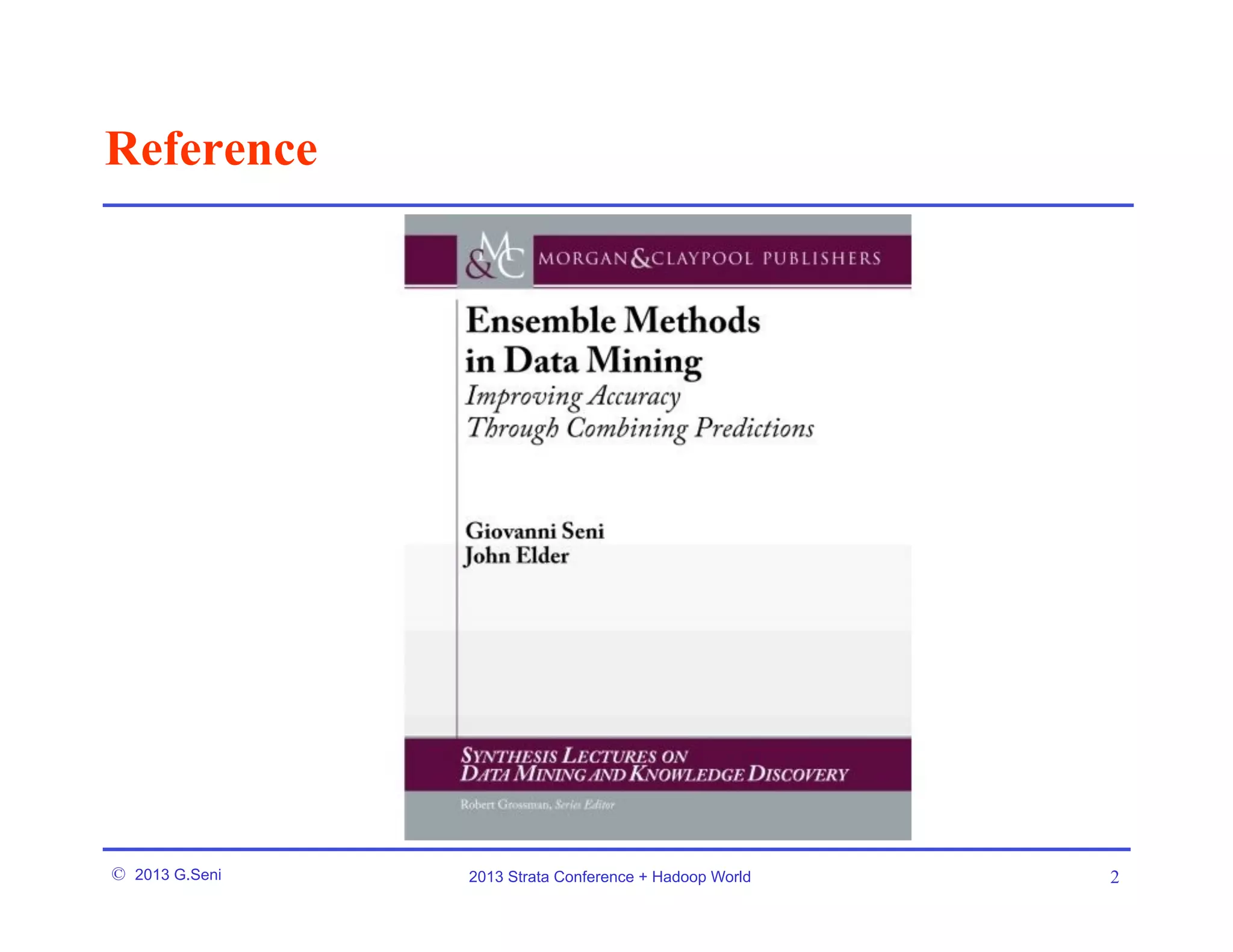
Book

•  Equivalence to Forward Stagewise Fitting Procedure
–  cm = arg min (⋅) is equivalent to line c.
c

•  R package adabag
© 2013 G.Seni


42

AdaBoost
Hands-on Exercise

1.0

• 

example.2.EllipticalBoundary
or with GUI

• 

Load and run

0.0

–  fitModel_Adaboost_by_hand.R

-0.5

• 

After class, load and run
fitModel_Adaboost.R and
fitModel_RandomForest.R

-1.0

x2

0.5

• 

-2

-1

0

1

2

x1

© 2013 G.Seni


43

Stochastic Gradient Boosting (Friedman, 2001)
•  Boosting with any differentiable loss criterion
ˆ
•  General L( y, y )

F0 (x) = c00

•  υ = 0.1 ⇒ Sequential sampling

For m = 1 to M {
(cm , p m ) = arg min
m
c, p

•  η = N 2

∑ηL( y , F
i

m −1

i∈S m ( )

(x i ) + c ⋅ T (x i ; p))

Tm (x) = T (x; p m )

•  Tm (x) ⇒ Any “weak” learner
N

•  co = arg minc ∑i =1 L( yi , c)

Fm (x) = Fm −1 (x) +υ ⋅ cm ⋅ Tm (x)
υ
}
M
write {(υ ⋅ cm ), Tm (x)}1

M
•  {cm }1 ⇒ “shrunk” sequential

partial regression coefficients

–  Potential improvements?
–  R package: gbm
© 2013 G.Seni


44

Stochastic Gradient Boosting
LAD Regression – L

!, ! = ! − !

•  More robust than ( y − F )2
•  Resistant to outliers in y
…trees already providing
resistance to outliers in x

!

N

F0 (x) = median{yi }1
For m = 1 to M {

// Step1 : find Tm (x)
~ = sign ( y − F (x ) )
yi
i
m −1
i

•  Note:


{R }

J

jm 1

–  Trees are fitted to pseudoresponse

(

// Step2 : find coefficients

⇒ Can’t interpret interpret

γˆ jm = median{yi − Fm −1 (x i )}1N

x i ∈R jm

individual trees

–  “shrunk” version of tree gets
added to ensemble

j = 1… J

// Update expansion

–  Original tree constants are
overwritten

© 2013 G.Seni

N
= J − terminal node LS - regression tree {~i , x i }1
y


Fm (x) = Fm −1 (x) + υ ⋅ ∑ γˆ jm I x i ∈ R jm
J

j =1

(

)

}


45

)

Parallel vs. Sequential Ensembles
100 Target Functions Comparison (Popescu, 2005)

Comparative RMS Error

•  xxx_6_5%_P : 6 terminal nodes trees
5% samples without replacement
Post-processing – i.e., using
estimated “optimal” quadrature
coefficients
“Sequential”

“Parallel”
Bag

RF

Boost

Seq_0.01_20%_P

•  Seq_υ_η%_P : “Sequential” ensemble
6 terminal nodes trees
υ : “memory” factor
η % samples without replacement
Post-processing

Bag_6_5%_P RF_6_5%_P
Seq_0.1_50%_P

•  Sequential ISLE tend to perform better than parallel ones
–  Consistent with results observed in classical Monte Carlo integration
© 2013 G.Seni


46

Rule Ensembles (Friedman & Popescu, 2005)
J

ˆ
ˆ
•  Trees as collection of conjunctive rules: Tm (x) = ∑ c jm I (x ∈ R jm )
j =1

R1

27

R4
15

R2 ⇒

R5
15

22

x1

r2 (x) = I ( x1 > 22) ⋅ I (0 ≤ x2 ≤ 27)
r3 (x) = I (15 < x1 ≤ 22) ⋅ I (0 ≤ x2 )

R4 ⇒

r4 (x) = I (0 ≤ x1 ≤ 15) ⋅ I ( x2 > 15)

R5 ⇒

x2

r1 (x) = I ( x1 > 22) ⋅ I ( x2 > 27)

R3 ⇒

R3

ˆ
y

R2

R1 ⇒

r5 (x) = I (0 ≤ x1 ≤ 15) ⋅ I (0 ≤ x2 ≤ 15)

–  These simple rules, rm (x) ∈ {0,1} can be used as base learners
,
–  Main motivation is interpretability
© 2013 G.Seni


47

Rule Ensembles
ISLE Procedure
•  Rule-based model: F (x) = a0 + ∑ am rm (x)
m

–  Still a piecewise constant model ⇒ complement the non-linear rules
with purely linear terms:

•  Fitting
–  Step 1: derive rules from tree ensemble (shortcut)
•  Tree size controls rule “complexity” (interaction order)

–  Step 2: fit coefficients using linear regularized procedure:

(

N
P
K
ˆ
ˆ
({ak },{b j }) = arg min ∑ L yi , F x; {ak }0 , {b j }1
{ak },{b j }

© 2013 G.Seni

i=1

(

)) +!!! ⋅


!(a) + !(b) !
48

Boosting & Rule Ensembles
Hands-on Exercise

2500

• 

example.3.Diamonds

Load and run

1500

or with GUI

• 

2000

• 

–  viewDiamondData.R
–  fitModel_GBM.R

1000

–  fitModel_RE.R
• 

500

Absolute loss


After class, go to:
example.1.LinearBoundary

0

200

400

600

800

1000

Run fitModel_GBM.R

Iteration

© 2013 G.Seni


49

Summary
•  Ensemble methods have been found to perform extremely
well in a variety of problem domains
•  Shown to have desirable statistical properties
•  Latest ensemble research brings together important
foundational strands of statistics
•  Emphasis on accuracy but significant progress has been
made on interpretability
Go build Ensembles and keep in touch!

© 2013 G.Seni


51

Strata 2013: Tutorial-- How to Create Predictive Models in R using Ensembles

More Related Content

What's hot

Viewers also liked

Similar to Strata 2013: Tutorial-- How to Create Predictive Models in R using Ensembles

More from Intuit Inc.

Recently uploaded

Strata 2013: Tutorial-- How to Create Predictive Models in R using Ensembles