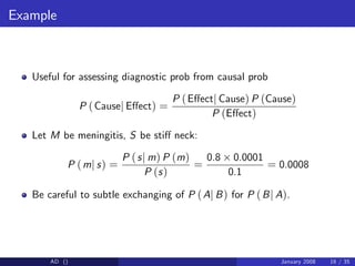
This document outlines the basics of probability and statistics as related to machine learning, covering concepts such as sample spaces, events, random variables, and probability distributions. It discusses important statistical principles including the Central Limit Theorem, Bayes' Rule, and maximum likelihood estimation, emphasizing both Bayesian and frequentist interpretations of probability. Various examples illustrate the application of these concepts in real-world scenarios, highlighting the significance of correct probabilistic reasoning.

1. CS 540: Machine Learning
Lecture 2: Review of Probability & Statistics
AD
January 2008
AD () January 2008 1 / 35

2. Outline
Probability “theory” (PRML, Section 1.2)
Statistics (PRML, Sections 2.1-2.4)
AD () January 2008 2 / 35

3. Probability Basics
Begin with a set Ω-the sample space; e.g. 6 possible rolls of a die.
ω 2 Ω is a sample point/possible event.
A probability space or probability model is a sample space with an
assignment P (ω) for every ω 2 Ω s.t.
0 P (ω) 1 and ∑
ω2Ω
P (ω) = 1;
e.g. for a die
P (1) = P (2) = P (3) = P (4) = P (5) = P (6) = 1/6.
An event A is any subset of Ω
P (A) = ∑
ω2A
P (ω)
e.g. P (die roll < 3) = P (1) + P (2) = 1/6 + 1/6 = 1/3.
AD () January 2008 3 / 35

4. Random Variables
A random variable is loosely speaking a function from sample points
to some range; e.g. the reals.
P induces a probability distribution for any r.v. X :
P (X = x) = ∑
fω2Ω:X (ω)=xg
P (ω)
e.g.
P (Odd = true) = P (1) + P (3) + P (5) = 1/6 + 1/6 + 1/6 = 1/2.
AD () January 2008 4 / 35

5. Why use probability?
“Probability theory is nothing but common sense reduced to
calculation” — Pierre Laplace, 1812.
In 1931, de Finetti proved that it is irrational to have beliefs that
violate these axioms, in the following sense:
If you bet in accordance with your beliefs, but your beliefs violate the
axioms, then you can be guaranteed to lose money to an opponent
whose beliefs more accurately re‡ect the true state of the world.
(Here, “betting” and “money” are proxies for “decision making” and
“utilities”.)
What if you refuse to bet? This is like refusing to allow time to pass:
every action (including inaction) is a bet.
Various other arguments (Cox, Savage).
AD () January 2008 5 / 35

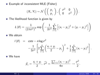
6. Probability for continuous variables
We typically do not work with probability distributions but with
densities.
We have
P (X 2 A) =
Z
A
pX (x) dx.
so Z
Ω
pX (x) dx = 1
We have
P (X 2 [x, x + δx]) pX (x) δx
Warning: A density evaluated at a point can be bigger than 1.
AD () January 2008 6 / 35

7. Univariate Gaussian (Normal) density
If X N µ, σ2 then the pdf of X is de…ned as
pX (x) =
1
p
2πσ2
exp
(x µ)2
2σ2
!
We often use the precision λ = 1/σ2 instead of the variance.
AD () January 2008 7 / 35

8. Statistics of a distribution
Recall that the mean and variance of a distribution are de…ned as
E (X) =
Z
xpX (x) dx
V (X) = E (X E (X))2
=
Z
(x E (X))2
pX (x) dx
For a Gaussian distribution, we have
E (X) = µ, V (X) = σ2
.
Chebyshev’
s inequality
P (jX E (X)j ε)
V (X)
ε2
.
AD () January 2008 8 / 35

9. Cumulative distribution function
The cumulative distribution function is de…ned as
FX (x) = P (X x) =
Z x
∞
pX (u) du
We have
lim
x! ∞
FX (x) = 0,
lim
x!∞
FX (x) = 1.
AD () January 2008 9 / 35

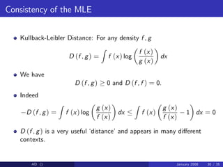
10. Law of large numbers
Assume you have Xi
i.i.d.
pX ( ) then
lim
n!∞
1
n
n
∑
i=1
ϕ (Xi ) = E [ϕ (X)] =
Z
ϕ (x) pX (x) dx
The result is still valid for weakly dependent random variables.
AD () January 2008 10 / 35

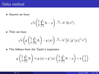
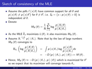
11. Central limit theorem
Let Xi
i.i.d.
pX ( ) such that E [Xi ] = µ and V (Xi ) = σ2 then
p
n
1
n
n
∑
i=1
Xi µ
!
D
! N 0, σ2
.
This result is (too) often used to justify the Gaussian assumption
AD () January 2008 11 / 35

12. Delta method
Assume we have
p
n
1
n
n
∑
i=1
Xi µ
!
D
! N 0, σ2
Then we have
p
n g
1
n
n
∑
i=1
Xi
!
g (µ)
!
D
! N 0, g0
(µ)
2
σ2
This follows from the Taylor’
s expansion
g
1
n
n
∑
i=1
Xi
!
g (µ) + g0
(µ)
1
n
n
∑
i=1
Xi µ
!
+ o
1
n
AD () January 2008 12 / 35

13. Prior probability
Consider the following random variables Sick2 fyes,nog and
Weather2 fsunny,rain,cloudy,snowg
We can set a prior probability on these random variables; e.g.
P (Sick = yes) = 1 P (Sick = no) = 0.1,
P (Weather) = (0.72, 0.1, 0.08, 0.1)
Obviously we cannot answer questions like
P (Sick = yesj Weather = rainy)
as long as we don’
t de…ne an appropriate distribution.
AD () January 2008 13 / 35

14. Joint probability distributions
We need to assign a probability to each sample point
For (Weather, Sick), we have to consider 4 2 events; e.g.
Weather / Sick sunny rainy cloudy snow
yes 0.144 0.02 0.016 0.02
no 0.576 0.08 0.064 0.08
From this probability distribution, we can compute probabilities of the
form P (Sick = yesj Weather = rainy) .
AD () January 2008 14 / 35

15. Bayes’rule
We have
P (x, y) = P (xj y) P (y) = P (yj x) P (x)
It follows that
P (xj y) =
P (x, y)
P (y)
=
P (yj x) P (x)
∑x P (yj x) P (x)
We have
P (Sick = yesj Weather = rainy) =
P (Sick = yes,Weather = rainy)
P (Weather = rainy)
=
0.02
0.02 + 0.08
= 0.2
AD () January 2008 15 / 35

16. Example
Useful for assessing diagnostic prob from causal prob
P (Causej E¤ect) =
P (E¤ectj Cause) P (Cause)
P (E¤ect)
Let M be meningitis, S be sti¤ neck:
P (mj s) =
P (sj m) P (m)
P (s)
=
0.8 0.0001
0.1
= 0.0008
Be careful to subtle exchanging of P (Aj B) for P (Bj A).
AD () January 2008 16 / 35

17. Example
Prosecutor’
s Fallacy. A zealous prosecutor has collected an evidence
and has an expert testify that the probability of …nding this evidence
if the accused were innocent is one-in-a-million. The prosecutor
concludes that the probability of the accused being innocent is
one-in-a-million.
This is WRONG.
AD () January 2008 17 / 35

18. Assume no other evidence is available and the population is of 10
million people.
De…ning A =“The accused is guilty” then P (A) = 10 7.
De…ning B =“Finding this evidence” then P (Bj A) = 1 &
P Bj A = 10 6.
Bayes formula yields
P (Aj B) =
P (Bj A) P (A)
P (Bj A) P (A) + P Bj A P A
=
10 7
10 7 + 10 6 (1 10 7)
0.1.
Real-life Example: Sally Clark was condemned in the UK (The RSS
pointed out the mistake). Her conviction was eventually quashed (on
other grounds).
AD () January 2008 18 / 35

19. You feel sick and your GP thinks you might have contracted a rare
disease (0.01% of the population has the disease).
A test is available but not perfect.
If a tested patient has the disease, 100% of the time the test will be
positive.
If a tested patient does not have the diseases, 95% of the time the test
will be negative (5% false positive).
Your test is positive, should you really care?
AD () January 2008 19 / 35

20. Let A be the event that the patient has the disease and B be the
event that the test returns a positive result
P (Aj B) =
1 0.0001
1 0.0001 + 0.05 0.9999
0.002
Such a test would be a complete waste of money for you or the
National Health System.
A similar question was asked to 60 students and sta¤ at Harvard
Medical School: 18% got the right answer, the modal response was
95%!
AD () January 2008 20 / 35

21. “General”Bayesian framework
Assume you have some unknown parameter θ and some data D.
The unknown parameters are now considered RANDOM of prior
density p (θ)
The likelihood of the observation D is p (Dj θ) .
The posterior is given by
p (θj D) =
p (Dj θ) p (θ)
p (D)
where
p (D) =
Z
p (Dj θ) p (θ) dθ
p (D) is called the marginal likelihood or evidence.
AD () January 2008 21 / 35

22. Bayesian interpretation of probability
In the Bayesian approach, probability describes degrees of belief,
instead of limiting frequencies.
The selection of a prior has an obvious impact on the inference
results! However, Bayesian statisticians are honest about it.
AD () January 2008 22 / 35

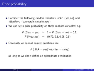
23. Bayesian inference involves passing from a prior p (θ) to a posterior
p (θj D) .We might expect that because the posterior incorporates the
information from the data, it will be less variable than the prior.
We have the following identities
E [θ] = E [E [θj D]] ,
V [θ] = E [V [θj D]] + V [E [θj D]] .
It means that, on average (over the realizations of the data X) we
expect the conditional expectation E [θj D] to be equal to E [θ] and
the posterior variance to be on average smaller than the prior variance
by an amount that depend on the variations in posterior means over
the distribution of possible data.
AD () January 2008 23 / 35

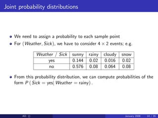
24. If (θ, X) are two scalar random variables then we have
V [θ] = E [V [θj D]] + V [E [θj D]] .
Proof:
V [θ] = E θ2
E (θ)2
= E E θ2
D (E (E (θj D)))2
= E E θ2
D E (E (θj D))2
+E (E (θj D))2
(E (E (θj D)))2
= E (V (θj X)) + V (E (θj X)) .
Such results appear attractive but one should be careful. Here there is
an underlying assumption that the observations are indeed distributed
according to p (D) .
AD () January 2008 24 / 35

25. Frequentist interpretation of probability
Probabilities are objective properties of the real world, and refer to
limiting relative frequencies (e.g. number of times I have observed
heads.).
Problem. How do you attribute a probability to the following event
“There will be a major earthquake in Tokyo on the 27th April 2013”?
Hence in most cases θ is assumed unknown but …xed.
We then typically compute point estimates of the form b
θ = ϕ (D)
which are designed to have various desirable quantities when averaged
over future data D0 (assumed to be drawn from the “true”
distribution).
AD () January 2008 25 / 35

26. Maximum Likelihood Estimation
Suppose we have Xi
i.i.d.
p ( j θ) for i = 1, ..., N then
L (θ) = p (Dj θ) =
N
∏
i=1
p (xi j θ) .
The MLE is de…ned as
b
θ = arg max L (θ)
= arg max l (θ)
where
l (θ) = log L (θ) =
N
∑
i=1
log p (xi j θ) .
AD () January 2008 26 / 35

27. MLE for 1D Gaussian
Consider Xi
i.i.d.
N µ, σ2 then
p Dj µ, σ2
=
N
∏
i=1
N xi ; µ, σ2
so
l (θ) =
N
2
log (2π)
N
2
log σ2 1
2σ2
N
∑
i=1
(xi µ)2
Setting
∂l(θ)
∂µ = ∂l(θ)
∂σ2 = 0 yields
b
µML =
1
N
N
∑
i=1
xi ,
c
σ2
ML =
1
N
N
∑
i=1
(xi b
µML)2
.
We have E [b
µML] = µ and E
h
c
σ2
ML
i
= N
N 1 σ2.
AD () January 2008 27 / 35

28. Consistent estimators
De…nition. A sequence of estimators b
θN = b
θN (X1, ..., XN ) is consistent
for the parameter θ if, for every ε > 0 and every θ 2 Θ
lim
N!∞
Pθ
b
θN θ < ε = 1 (equivalently lim
N!∞
Pθ
b
θN θ ε = 0).
Example: Consider Xi
i.i.d.
N (µ, 1) and b
µN = 1
N ∑N
i=1 Xi then
b
µN N µ, N 1 and
Pθ
b
θN θ < ε =
Z ε
p
N
ε
p
N
1
p
2π
exp
u2
2
du ! 1.
It is possible to avoid this calculations and use instead Chebychev’
s
inequality
Pθ
b
θN θ ε = Pθ
b
θn θ
2
ε2
Eθ
b
θn θ
2
ε2
where Eθ
b
θn θ
2
= varθ
b
θn + Eθ
b
θn θ
2
.
AD () January 2008 28 / 35

29. Example of inconsistent MLE (Fisher)
(Xi , Yi ) N
µi
µi
,
σ2 0
0 σ2 .
The likelihood function is given by
L (θ) =
1
(2πσ2)n exp
1
2σ2
n
∑
i=1
h
(xi µi )2
+ (yi µi )2
i
!
We obtain
l (θ) = cste n log σ2
1
2σ2
"
2
n
∑
i=1
xi + yi
2
µi
2
+
1
2
n
∑
i=1
(xi yi )2
#
.
We have
b
µi =
xi + yi
2
, c
σ2 =
∑n
i=1 (xi yi )2
4n
!
σ2
2
.
AD () January 2008 29 / 35

30. Consistency of the MLE
Kullback-Leibler Distance: For any density f , g
D (f , g) =
Z
f (x) log
f (x)
g (x)
dx
We have
D (f , g) 0 and D (f , f ) = 0.
Indeed
D (f , g) =
Z
f (x) log
g (x)
f (x)
dx
Z
f (x)
g (x)
f (x)
1 dx = 0
D (f , g) is a very useful ‘
distance’and appears in many di¤erent
contexts.
AD () January 2008 30 / 35

31. Sketch of consistency of the MLE
Assume the pdfs f (xj θ) have common support for all θ and
p (xj θ) 6= p xj θ0
for θ 6= θ0
; i.e. Sθ = fx : p (xj θ) > 0g is
independent of θ.
Denote
MN (θ) =
1
N
N
∑
i=1
log
p (Xi j θ)
p (Xi j θ )
As the MLE b
θn maximizes L (θ), it also maximizes MN (θ) .
Assume Xi
i.i.d.
p ( j θ ). Note that by the law of large numbers
MN (θ) converges to
Eθ log
p (Xj θ)
p (Xj θ )
=
Z
p (xj θ ) log
p (xj θ)
p (xj θ )
dx
= D (p ( j θ ) , p ( j θ)) := M (θ) .
Hence, MN (θ) D (p ( j θ ) , p ( j θ)) which is maximized for θ
so we expect that its maximizer will converge towards θ .
AD () January 2008 31 / 35

32. Asymptotic Normality
Assuming b
θN is a consistent estimate of θ , we have under regularity
assumptions
p
N b
θN θ ) N 0, [I (θ )] 1
where
[I (θ)]k,l = E
∂2 log p (xj θ)
∂θk ∂θl
We can estimate I (θ ) through
[I (θ )]k,l =
1
N
N
∑
i=1
∂2 log p (Xi j θ)
∂θk ∂θl b
θN
AD () January 2008 32 / 35

33. Sketch of the proof
We have
0 = l0 b
θN l0
(θ ) + b
θN θ l00
(θ )
)
p
N b
θN θ =
1
p
N
l0 (θ )
1
N l00 (θ )
Now l0 (θ ) = ∑n
i=1
∂ log p( Xi jθ)
∂θ θ
where Eθ
h
∂ log p( Xi jθ)
∂θ θ
i
= 0 and
varθ
h
∂ log p( Xi jθ)
∂θ θ
i
= I (θ ) so the CLT tells us that
1
p
N
l0
(θ )
D
! N (0, I (θ ))
where by the law of large numbers
1
N
l00
(θ ) =
1
N
N
∑
i=1
∂2 log p (Xi j θ)
∂θk ∂θl θ
! I (θ ) .
AD () January 2008 33 / 35

34. Frequentist con…dence intervals
The MLE being approximately Gaussian, it is possible to de…ne
(approximate) con…dence intervals.
However be careful, “θ has a 95% con…dence interval of [a, b]” does
NOT mean that P (θ 2 [a, b]j D) = 0.95.
It means
PD0 P( jD) θ 2 a D0
, b D0
= 0.95
i.e., if we were to repeat the experiment, then 95% of the time, the
true parameter would be in that interval. This does not mean that we
believe it is in that interval given the actual data D we have observed.
AD () January 2008 34 / 35

35. Bayesian statistics as an unifying approach
In my opinion, the Bayesian approach is much simpler and more
natural than classical statistics.
Once you have de…ned a Bayesian model, everything follows naturally.
De…ning a Bayesian model requires specifying a prior distribution, but
this assumption is clearly stated.
For many years, Bayesian statistics could not be implemented for all
but the simple models but now numerous algorithms have been
proposed to perform approximate inference.
AD () January 2008 35 / 35