Download as PDF, PPTX

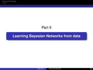
![Introduction
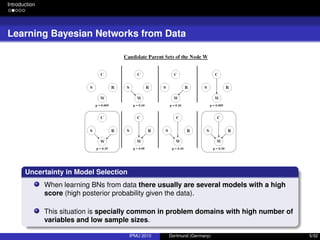
Integration of Expert Knowledge
Expert Knowledge
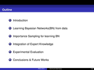
In many domain problems expert knowledge is available.
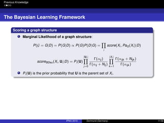
The graphical structure of BNs greatly ease the interaction with a human expert:
Causal ordering.
D-separtion criteria.
Previous Works I
There have been many attempts to introduce expert knowledge when learning
BNs from data.
Via Prior Distribution [2,5]: Use of specific prior distributions over the
possible graph structures to integrate expert knowledge:
Expert assigns higher prior probabilities to most likely edges.
IPMU 2010 Dortmund (Germany) 6/32](https://image.slidesharecdn.com/slides-intercativelearning-ipmu-151124194045-lva1-app6891/85/An-Importance-Sampling-Approach-to-Integrate-Expert-Knowledge-When-Learning-Bayesian-Networks-From-Data-7-320.jpg)
![Introduction
Integration of Expert Knowledge
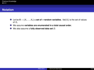
Previous Works II
Via structural Restrictions [6]: Expert codify his/her knowledge as structural
restrictions.
Expert defines the existence/absence of arcs and/or edges and causal
ordering restrictions.
Retrieved model should satisfy these restrictions.
IPMU 2010 Dortmund (Germany) 7/32](https://image.slidesharecdn.com/slides-intercativelearning-ipmu-151124194045-lva1-app6891/85/An-Importance-Sampling-Approach-to-Integrate-Expert-Knowledge-When-Learning-Bayesian-Networks-From-Data-8-320.jpg)
![Introduction
Integration of Expert Knowledge
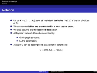
Previous Works II
Via structural Restrictions [6]: Expert codify his/her knowledge as structural
restrictions.
Expert defines the existence/absence of arcs and/or edges and causal
ordering restrictions.
Retrieved model should satisfy these restrictions.
Limitations of "Prior" Expert Knowledge
The system would ask to the expert his/her belief about any possible feature
of the BN (non feasible in high domains).
The expert could be biased to provide the most “easy” or clear knowledge.
The system does not help to the user to introduce information about the BN
structure.
IPMU 2010 Dortmund (Germany) 7/32](https://image.slidesharecdn.com/slides-intercativelearning-ipmu-151124194045-lva1-app6891/85/An-Importance-Sampling-Approach-to-Integrate-Expert-Knowledge-When-Learning-Bayesian-Networks-From-Data-9-320.jpg)
![Previous Knowledge
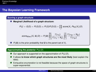
Approximating the Posterior P(Ui|D)
Closed Form Solution
In [3] it was proposed a closed form solution assuming a node can have up to
K parents.
It would have a polynomial efficiency O(n(K+1)).
IPMU 2010 Dortmund (Germany) 13/32](https://image.slidesharecdn.com/slides-intercativelearning-ipmu-151124194045-lva1-app6891/85/An-Importance-Sampling-Approach-to-Integrate-Expert-Knowledge-When-Learning-Bayesian-Networks-From-Data-19-320.jpg)
![Previous Knowledge
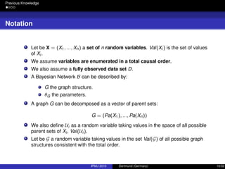
Approximating the Posterior P(Ui|D)
Closed Form Solution
In [3] it was proposed a closed form solution assuming a node can have up to
K parents.
It would have a polynomial efficiency O(n(K+1)).
Markov Chain Monte Carlo
Lets Val(Ui ) be the space model of the Markov Chain.
If the Markov Chain is in some state U in iteration t, a new model U is
randomly drawn by adding, deleting of switching any edge.
The Markov Chain moves to state U in the iteration t + 1 with probability:
m(Ut
, Ut+1
) = min{1,
N(U)score(D|U )
N(U )score(D|U)
}
If it not, the Markov Chain remains in state U.
This Markov Chain has an stationary distribution (t → ∞) which is P(U|D).
IPMU 2010 Dortmund (Germany) 13/32](https://image.slidesharecdn.com/slides-intercativelearning-ipmu-151124194045-lva1-app6891/85/An-Importance-Sampling-Approach-to-Integrate-Expert-Knowledge-When-Learning-Bayesian-Networks-From-Data-20-320.jpg)

![Integrating Expert Knowledge
Prior Knowledge
Representing absence of prior knowledge
“Uniform prior over structures is usually chosen by convenience” [3].
P(G) does not grow with the data, but it matters at low sample sizes.
IPMU 2010 Dortmund (Germany) 22/32](https://image.slidesharecdn.com/slides-intercativelearning-ipmu-151124194045-lva1-app6891/85/An-Importance-Sampling-Approach-to-Integrate-Expert-Knowledge-When-Learning-Bayesian-Networks-From-Data-31-320.jpg)
![Integrating Expert Knowledge
Prior Knowledge
Representing absence of prior knowledge
“Uniform prior over structures is usually chosen by convenience” [3].
P(G) does not grow with the data, but it matters at low sample sizes.
Let us assume that the prior probability of an edge is p and independent of
each other. If Xi has k parents out of m nodes:
P(Pa(Xi )) = pk
(1 − p)(m−k)
If the number of candidate parents m grows, p should be decreased to
control de number of false positives edges: “multiplicity correction”.
IPMU 2010 Dortmund (Germany) 22/32](https://image.slidesharecdn.com/slides-intercativelearning-ipmu-151124194045-lva1-app6891/85/An-Importance-Sampling-Approach-to-Integrate-Expert-Knowledge-When-Learning-Bayesian-Networks-From-Data-32-320.jpg)
![Integrating Expert Knowledge
Prior Knowledge
Representing absence of prior knowledge
“Uniform prior over structures is usually chosen by convenience” [3].
P(G) does not grow with the data, but it matters at low sample sizes.
Let us assume that the prior probability of an edge is p and independent of
each other. If Xi has k parents out of m nodes:
P(Pa(Xi )) = pk
(1 − p)(m−k)
If the number of candidate parents m grows, p should be decreased to
control de number of false positives edges: “multiplicity correction”.
This is solved by assuming that p has a Beta prior with parameter α = 0.5 [11]:
Pi (Pa(Xi )) =
Γ(2 ∗ α)
Γ(m + 2α)
Γ(k + α)Γ(m − k + α)
Γ(α)Γ(α)
IPMU 2010 Dortmund (Germany) 22/32](https://image.slidesharecdn.com/slides-intercativelearning-ipmu-151124194045-lva1-app6891/85/An-Importance-Sampling-Approach-to-Integrate-Expert-Knowledge-When-Learning-Bayesian-Networks-From-Data-33-320.jpg)
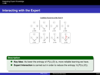
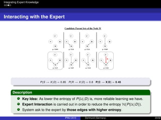
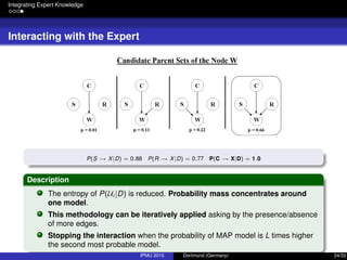

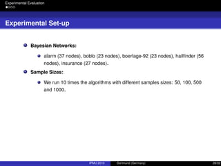
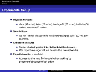
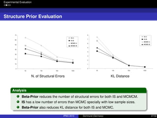
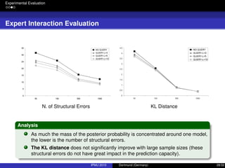
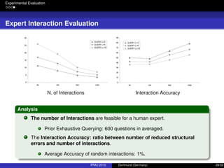


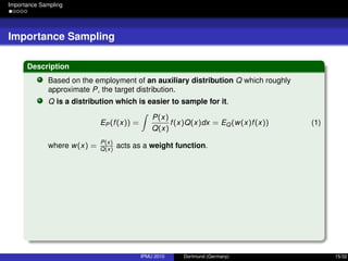
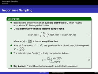
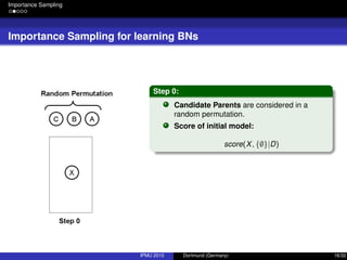
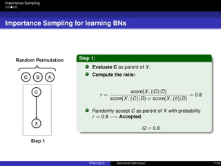
The document discusses integrating expert knowledge into the learning of Bayesian networks using an importance sampling approach, addressing challenges like model uncertainty and sample size limitations. It outlines methodologies for interactive learning, emphasizing the need for expert input to refine models and reduce entropy for better predictions. Experimental evaluations demonstrate how using structured expert knowledge can improve learning outcomes, particularly in conditions of limited data.


![Introduction to bayesian_networks[1]](https://cdn.slidesharecdn.com/ss_thumbnails/introductiontobayesiannetworks1-150525024327-lva1-app6891-thumbnail.jpg?width=640&height=640&fit=bounds)


![Polymer [ बहुलक ] Chemistry Notes PDF - Irfanullah Mehar - JJ Sir Chemistry.pdf](https://cdn.slidesharecdn.com/ss_thumbnails/polymerchemistrynotespdf-irfanullahmehar-jjsirchemistry-260210172118-3f9b37f7-thumbnail.jpg?width=640&height=640&fit=bounds)


![ANIMAL_CELL_,_TISSUE_AND_ORGAN_CULTURE[1].pptx](https://cdn.slidesharecdn.com/ss_thumbnails/animalcelltissueandorganculture1-260204172026-4462b440-thumbnail.jpg?width=640&height=640&fit=bounds)


