The document discusses Monte Carlo methods for simulating systems in statistical mechanics, focusing on the Metropolis algorithm for sampling configurations in the canonical ensemble. It details the step-by-step process of generating new configurations, calculating energy changes, and using acceptance criteria based on these energy differences. Additionally, it covers related topics such as ergodicity, heat capacity, and order-disorder transitions, emphasizing the need for periodic boundary conditions in simulations.

1. Monte Carlo Methods:
- Markov Chain
Random movements, one follow another
- Importance sampling
To sample many points in the region where the Boltzmann
factor is large and few elsewhere
- Ergodicity (ensemble average)
Such an average over all possible quantum states of a system
- Detailed Balance
?
?
Metropolis Method:
]/)(exp[yprobabilithaccept wit:
accept:
TKEEEE
EE
Bonon
on
−−>
<

2. In terms of words:
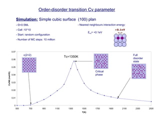
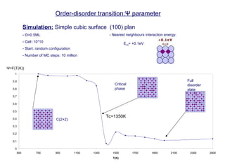
- Canonical ensemble: N,V,T constant
- Metropolis method: To generate a new configuration with probabilities
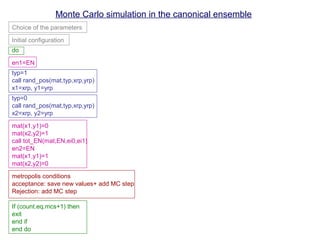
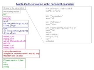
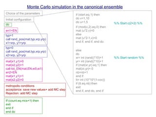
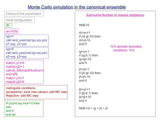
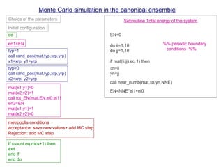
Monte Carlo simulation in the canonical ensemble
0. Generate the initial configuration (random or c(2×2))
Beginning of the MC cycle
1. Calculate Eold
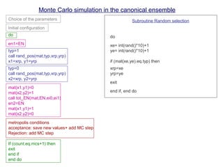
2. Randomly select a particle
3. Random displacement (or rotation)
4. Calculate Enew
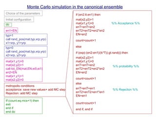
5. Accept the move with probability (Metropolis method)
En<Eo accept (the move)
En>Eo accept with probability exp[-(En-Eo)/kT]
(Periodic boundary conditions)
End of MC cycle

3. In terms of diagram:
Monte Carlo simulation in the canonical ensemble

4. Monte Carlo simulation in the canonical ensemble
Choice of the parameters
Initial configuration
do
en1=EN
typ=1
call rand_pos(mat,typ,xrp,yrp)
x1=xrp, y1=yrp
typ=0
call rand_pos(mat,typ,xrp,yrp)
x2=xrp, y2=yrp
mat(x1,y1)=0
mat(x2,y2)=1
mat(x1,y1)=1
mat(x2,y2)=0
call tot_EN(mat,EN,ei0,ei1)
en2=EN
metropolis conditions
acceptance: save new values+ add MC step
Rejection: add MC step
If (count.eq.mcs+1) then
exit
end if
end do

5. Monte Carlo simulation in the canonical ensemble
Choice of the parameters
Initial configuration
do
en1=EN
typ=1
call rand_pos(mat,typ,xrp,yrp)
x1=xrp, y1=yrp
typ=0
call rand_pos(mat,typ,xrp,yrp)
x2=xrp, y2=yrp
mat(x1,y1)=0
mat(x2,y2)=1
mat(x1,y1)=1
mat(x2,y2)=0
call tot_EN(mat,EN,ei0,ei1)
en2=EN
metropolis conditions
acceptance: save new values+ add MC step
Rejection: add MC step
If (count.eq.mcs+1) then
exit
end if
end do
real, parameter:: k=8,617339E-5
real *8:: enT,enT2
print *,”temperature:”
read(*,*) T
print *,”MC steps:”
read(*,*) mcs
print *,”starting configuration, R or C:”
read(*,*) st
start=0
select case (st)
case ( “c”, “C”)
start=1
end select

6. Monte Carlo simulation in the canonical ensemble
Choice of the parameters
Initial configuration
do
en1=EN
typ=1
call rand_pos(mat,typ,xrp,yrp)
x1=xrp, y1=yrp
typ=0
call rand_pos(mat,typ,xrp,yrp)
x2=xrp, y2=yrp
mat(x1,y1)=0
mat(x2,y2)=1
mat(x1,y1)=1
mat(x2,y2)=0
call tot_EN(mat,EN,ei0,ei1)
en2=EN
metropolis conditions
acceptance: save new values+ add MC step
Rejection: add MC step
If (count.eq.mcs+1) then
exit
end if
end do
if (start.eq.1) then
do v=1,10
if (mod(v,2).eq.0) then
mat (u*2,v)=0
else
mat (u*2-1,v)=0
end if, end if, end do
else
do
xr= int (rand()*10)+1
yr= int (rand()*10)+1
if (mat(xr,yr).eq.1) then
mat(xr,yr)= 0
do u=1,5
nb=nb+1
end if
tt= int (10*10*(1-cov))
if (tt.eq.nb) then
exit
end if, end do, end if
%% Start c(2×2) %%
%% Start random %%

7. Monte Carlo simulation in the canonical ensemble
Choice of the parameters
Initial configuration
do
en1=EN
typ=1
call rand_pos(mat,typ,xrp,yrp)
x1=xrp, y1=yrp
typ=0
call rand_pos(mat,typ,xrp,yrp)
x2=xrp, y2=yrp
mat(x1,y1)=0
mat(x2,y2)=1
mat(x1,y1)=1
mat(x2,y2)=0
call tot_EN(mat,EN,ei0,ei1)
en2=EN
metropolis conditions
acceptance: save new values+ add MC step
Rejection: add MC step
If (count.eq.mcs+1) then
exit
end if
end do
if (en2.lt.en1) then
mat(x2,y2)=1
enT=enT+en2
enT2=enT2+en2*en2
count=count+1
else
if (exp(-(en2-en1)/(k*T)).gt.rand()) then
mat(x2,y2)=1
mat(x1,y1)=0
enT=enT+en2
enT2=enT2+en2*en2
count=count+1
mat(x1,y1)=0
else
end if, end if
enT=enT+en1
enT2=enT2+en1*en1
EN=en1
count=count+1
EN=en2
EN=en2
%% Acceptance %%
%% probability %%
%% Rejection %%

8. Monte Carlo simulation in the canonical ensemble
Choice of the parameters
Initial configuration
do
en1=EN
typ=1
call rand_pos(mat,typ,xrp,yrp)
x1=xrp, y1=yrp
typ=0
call rand_pos(mat,typ,xrp,yrp)
x2=xrp, y2=yrp
mat(x1,y1)=0
mat(x2,y2)=1
mat(x1,y1)=1
mat(x2,y2)=0
call tot_EN(mat,EN,ei0,ei1)
en2=EN
metropolis conditions
acceptance: save new values+ add MC step
Rejection: add MC step
If (count.eq.mcs+1) then
exit
end if
end do
Subroutine Number of nearest neighbours
NNE=0
id=xn+1
if (id.gt.10) then
end if
ig=xn-1
if (ig.lt.1) then
ig=ig+10
end if
jh=yn-1
if (jh.gt.10) then
jh=jh-10
end if
jb=yn+1
if (jb.lt.1) then
jb=jb+10
end if
NNE=id + ig + jb + jh
%% periodic boundary
conditions %%
id=id-10

9. Monte Carlo simulation in the canonical ensemble
Choice of the parameters
Initial configuration
do
en1=EN
typ=1
call rand_pos(mat,typ,xrp,yrp)
x1=xrp, y1=yrp
typ=0
call rand_pos(mat,typ,xrp,yrp)
x2=xrp, y2=yrp
mat(x1,y1)=0
mat(x2,y2)=1
mat(x1,y1)=1
mat(x2,y2)=0
call tot_EN(mat,EN,ei0,ei1)
en2=EN
metropolis conditions
acceptance: save new values+ add MC step
Rejection: add MC step
If (count.eq.mcs+1) then
exit
end if
end do
Subroutine Total energy of the system
EN=0
do ii=1,10
do jj=1,10
if mat(ii,jj).eq.1) then
%% periodic boundary
conditions %%
xn=ii
yn=jj
call near_numb(mat,xn,yn,NNE)
EN=NNE*ei1+ei0

10. Monte Carlo simulation in the canonical ensemble
Choice of the parameters
Initial configuration
do
en1=EN
typ=1
call rand_pos(mat,typ,xrp,yrp)
x1=xrp, y1=yrp
typ=0
call rand_pos(mat,typ,xrp,yrp)
x2=xrp, y2=yrp
mat(x1,y1)=0
mat(x2,y2)=1
mat(x1,y1)=1
mat(x2,y2)=0
call tot_EN(mat,EN,ei0,ei1)
en2=EN
metropolis conditions
acceptance: save new values+ add MC step
Rejection: add MC step
If (count.eq.mcs+1) then
exit
end if
end do
Subroutine Random selection
do
xe= int(rand()*10)+1
ye= int(rand()*10)+1
if (mat(xe,ye).eq.typ) then
xrp=xe
yrp=ye
exit
end if, end do

11. Monte Carlo simulation in the canonical ensemble
Choice of the parameters
Initial configuration
do
en1=EN
typ=1
call rand_pos(mat,typ,xrp,yrp)
x1=xrp, y1=yrp
typ=0
call rand_pos(mat,typ,xrp,yrp)
x2=xrp, y2=yrp
mat(x1,y1)=0
mat(x2,y2)=1
mat(x1,y1)=1
mat(x2,y2)=0
call tot_EN(mat,EN,ei0,ei1)
en2=EN
metropolis conditions
acceptance: save new values+ add MC step
Rejection: add MC step
If (count.eq.mcs+1) then
exit
end if
end do
Subroutine Order parameter
matf=mat*2-1
do r = 1,10
do q = 1,5
if (mod(r,2).eq.0) then
ma=ma+matf(2*q-1,r)
mb=mb+matf(2*q,r)
else
ma=ma+matf(2*q,r)
mb=mb+matf(2*q-1,r)
end if, end do, end do
Psi=sqrt((ma-mb)*(ma-mb)/100
Subroutine Heat capacity parameter
cv = ((enT2/mcs)-(enT*enT) / (mcs*mcs))) / (k*T*T)

12. Order-disorder transition Cv parameter
0
0.01
0.02
0.03
0.04
0.05
0.06
0.07
500 700 900 1100 1300 1500 1700 1900 2100 2300 2500
T(K)
Cv/N0(meV/K)
Tc=1350K
Simulation: Simple cubic surface (100) plan
- Θ=0.5ML
- Cell :10*10
- Start: random configuration
- Number of MC steps: 10 million
c(2×2)
Critical
phase
Full
disorder
state
- Nearest neighbours interaction energy:
Eint= +0.1eV

13. 0
0.1
0.2
0.3
0.4
0.5
0.6
0.7
0.8
0.9
1
500 700 900 1100 1300 1500 1700 1900 2100 2300 2500
T(K)
Order-disorder transition:Ψ parameter
Simulation: Simple cubic surface (100) plan
- Θ=0.5ML
- Cell :10*10
- Start: random configuration
- Number of MC steps: 10 million
Tc=1350K
C(2×2)
Critical
phase
Full
disorder
state
- Nearest neighbours interaction energy:
Eint= +0.1eV
Ψ=F(T(K))