This document discusses survival analysis and Cox regression for cancer clinical trials. It begins with an introduction to Cox regression analysis and how it can be used to analyze the effects of covariates on survival rates in cancer trials. The document then provides examples of Cox regression outputs and how to interpret the results, including checking the proportional hazards assumption. It cautions against some invalid methods of survival analysis that do not properly account for censored or time-dependent data.

1. Survival Analysis and Cox
Regression for Cancer Trials
Presented at PG Department of Statistics,
Sardar Patel University January 29, 2013
Dr. Bhaswat S. Chakraborty
Sr. VP & Chair, R&D Core Committee
Cadila Pharmaceuticals Ltd., Ahmedabad
1

2. Part 2: Cox Regression
Analysis of Cancer CTs
2

3. Clinical Trials
 Organized scientific efforts to get direct answers from
relevant patients on important scientific questions on
(doses and regimens of) actions of drugs (or devices or
other interventions).
 Questions are mainly about differences or null
 Modern trials (last 40 years or so) are large, multicentre,
often international and co-operative endeavors
 Ideally, primary objectives are consistent with mechanism
of action
 Results can be translated to practice
 Would stand the regulatory and scientific scrutiny
3

4. Cancer Trials (Phases I–IV)
 Highly complex trials involving cytotoxic drugs, moribund patients,
time dependent and censored variables
 Require prolonged observation of each patient
 Expensive, long term and resource intensive trials
 Heterogeneous patients at various stages of the disease
 Prognostic factors of non-metastasized and metastasized diseases are
different
 Adverse reactions are usually serious and frequently include death
 Ethical concerns are numerous and very serious
 Trial management is difficult and patient recruitment extremely
challenging
 Number of stopped trials (by DSMB or FDA) is very high
 Data analysis and interpretation are very difficult by any standard
5

5. 6
Source: WHO

6. 7

7. India: 2010
 7137 of 122 429 study deaths were due to cancer, corresponding to 556 400 national
cancer deaths in India in 2010.
 395 400 (71%) cancer deaths occurred in people aged 30—69 years (200 100 men
and 195 300 women).
 At 30—69 years, the three most common fatal cancers were oral (including lip and
pharynx, 45 800 [22·9%]), stomach (25 200 [12·6%]), and lung (including trachea
and larynx, 22 900 [11·4%]) in men, and cervical (33 400 [17·1%]), stomach
(27 500 [14·1%]), and breast (19 900 [10·2%]) in women.
 Tobacco-related cancers represented 42·0% (84 000) of male and 18·3% (35 700) of
female cancer deaths and there were twice as many deaths from oral cancers as lung
cancers.
 Age-standardized cancer mortality rates per 100 000 were similar in rural (men 95·6
[99% CI 89·6—101·7] and women 96·6 [90·7—102·6]) and urban areas (men 102·4
[92·7—112·1] and women 91·2 [81·9—100·5]), but varied greatly between the
states.
 Cervical cancer was far less common in Muslim than in Hindu women (study deaths
24, age-standardized mortality ratio 0·68 [0·64—0·71] vs 340, 1·06 [1·05—1·08]).
8

8. 10

9. Survival Analysis
 Survival analysis is studying the time between entry
to a study and a subsequent event (such as death).
 Also called “time to event analysis”
 Survival analysis attempts to answer questions such
as:
 which fraction of a population will survive past a certain
time ?
 at what rate will they fail ?
 at what rate will they present the event ?
 How do particular factors benefit or affect the probability of
survival ?
11

10. What kind of time to event data?
 Survival Analysis typically focuses on time to event data.
 In the most general sense, it consists of techniques for
positive-valued random variables, such as
 time to death
 time to onset (or relapse) of a disease
 length of stay in a hospital
 money paid by health insurance
 viral load measurements
 Kinds of survival studies include:
 clinical trials
 prospective cohort studies
 retrospective cohort studies
 retrospective correlative studies
12

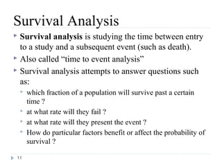
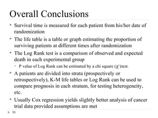
11. Definition and Characteristics of Variables
 Survival time (t) random variables (RVs) are always non-
negative, i.e., t ≥ 0.
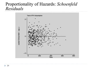
 T can either be discrete (taking a finite set of values, e.g.
a1, a2, …, an) or continuous [defined on (0,∞)].
 A random variable t is called a censored survival time RV
if x = min(t, u), where u is a non-negative censoring
variable.
 For a survival time RV, we need:
 (1) an unambiguous time origin (e.g. randomization to clinical
trial)
 (2) a time scale (e.g. real time (days, months, years)
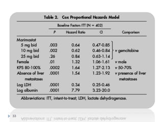
 (3) defnition of the event (e.g. death, relapse)
13

12. Event
Test
Non-Event
Sample of Target Randomize
Population
Event
Control
Non-Event
Time to Event
14

13. Illustration of Survival Data
15

14. Why Regression for Survival Data?
 Survival, in the form of hazard function, and one or more
explanatory co-variables can be very interesting research
investigation
 The relation with risk factors can be studied using group-
specific Kaplan-Meier estimates, together with Logrank and/or
Wilcoxon tests
 Investigating the relation with covariates, requires a
regression-type model
 Relating the outcome to several factors and/or covariates
simultaneously requires multiple regression, ANOVA, or
ANCOVA models
 The most frequently used model is the Cox (proportional
hazards) model
16

15. Understanding the Effect of Co-variables
17

16. Cox Proportional Hazards Regression
 Most common Cox are linear-like models for the log
hazard
 For example, a parametric regression model based on the
exponential distribution:
loge hi(t) = α + β1xi1 + β2xi2 + … + βkxik
 or, equivalently,
hi(t) = exp (α + β1xi1 + β2xi2 + … + βkxik)
= eα x eβ1xi1 x eβ2xi2 x … x eβkxik
 Where
 i indexes subjects and
 xi1, xi2, …, xik are the values of the co-variates for the ith
18
subject

17. Cox Model contd..
 This is therefore a linear model for the log-hazard or a multiplicative
model for the hazard itself
 The model is parametric because, once the regression parameters α,
β1, … βk are specified, the hazard function hi(t) is fully characterized by
the model
 The regression constant α represents a kind of baseline hazard, since
loge hi(t) = α, or equivalently, hi(t) = eα, when all of the x’s are 0
 Other parametric hazard regression models are based on other
distributions commonly used in modeling survival data, such as the
Gompertz and Weibull distributions.
 Parametric hazard models can be estimated with standards softwares
19
Source: John Fox

18. Cox Regression is a Proportional Hazards
Model
 Consider two observations, h1(t): hazard for the experimental group and
h0(t): hazard for the control group
h1(t)/h0(t) = exp(β)
 exp (β) indicates how large (small) is the hazard in experimental group with
the respect to the hazard in the reference group
 and it is constant, does not depend on time. Hence, it is called “proportional
hazards” over time
 Other qualities:
 Usually provides better estimates of survival probabilities and
cumulative hazard than those provided by the Kaplan-Meier function
when assumptions are met
 The coefficients in a Cox regression relate to hazard
 a positive coefficient indicates a worse prognosis
 a negative coefficient indicates a protective effect of the variable with which it is
associated
20

19. Exploring Co-variables by Cox Regression
21 Source: Yesilda Balavarca, Internet

20. Interpretation of Results
h1 (t,X) = h0(t) exp (β1 gender + β2 treatment)
 Gender: 1 = male, 0 = female; treament: 1 = experimental,
0 = control
h1 (t,X) = h0(t) exp (−0.51 gender + 0.69 treatment) and
exp(β1 ) = exp(−0.51 ) = 0.6 and exp(β2 ) = exp(0.69 ) = 2.0
 This means a reduction of hazards for males, i.e., males have
larger probabilities of survival than females
 The experimental treatment increases hazard, i.e., patients
receiving the new experimental treatment have lower survival
probabilities than patients on the control (standard) treatment
22

21. Checking Proportionality of Hazards
 Check to see if the estimated survival curves cross
 If they do, then this is evidence that the hazards are not
proportional
 More formal test: e.g., scaled Schoenfeld Residuals show
interactions between covariates and time
 Testing the time dependent covariates is equivalent to testing
for a non-zero slope in a generalized linear regression of the
scaled Schoenfeld residuals on functions of time
 A non-zero slope is an indication of a violation of the
proportional hazard assumption.
23

22. Proportionality of Hazards: Schoenfeld
Residuals
24

23. Cox Regression is a Proportional Hazards
Model
 Cox regression (or proportional hazards regression) is method
for investigating the effect of several variables upon the time a
specified event takes to happen
 When an outcome is death this is known as Cox regression for
survival analysis
 Assumptions:
 the effects of the predictor variables upon survival are constant over time
 are additive in one scale
 Usually provides better estimates of survival probabilities and
cumulative hazard than those provided by the Kaplan-Meier
function when assumptions are met
 The coefficients in a Cox regression relate to hazard
 a positive coefficient indicates a worse prognosis
 a negative coefficient indicates a protective effect of the variable with
which it is associated
25

24. Remember the Survival Data in
Part 1?
26

25. Organized Input Data
Group Surv Time Surv Censor Surv Group Surv Time Surv Censor Surv
2 142 1 2 232 1
1 143 1 2 232 1
2 157 1 2 232 1
2 163 1 2 233 1
1 165 1 2 233 1
1 188 1 2 233 1
1 188 1 2 233 1
1 235 1
1 190 1 2 239 1
1 192 1 2 240 1
2 198 1 1 244 0
2 204 0 1 246 1
2 205 1 2 261 1
1 206 1 1 265 1
1 208 1 2 280 1
1 212 1 2 280 1
1 216 0 2 295 1
1 216 1 2 295 1
1 220 1 1 303 1
1 227 1 2 323 1
1 230 1 2 344 0
27

26. Hazard Rate Plot
28

27. Log Hazard Plot
29

28. Cox Hazard Analysis
95% Conf. Hazard =
Coefficient (±) Std.Error P Exp(Coef.)
Group
Surv -0.5861172 0.6726008 0.343165 0.0876 0.55648
The significance test for the coefficient b1 tests the null hypothesis that it
equals zero and thus that its exponent equals one
The confidence interval for b1 is therefore the confidence interval for the
relative death rate or hazard ratio
What is your conclusion of this analysis?
30

29. And the Case Study Data in
Part 1?
31

30. Case Study: Results
 Cox proportional hazards:
 Factors associated with increased mortality risk were male
sex, poor KPS (< 80), presence of liver metastases, high
serum lactate dehydrogenase, and low serum albumin.
 Adjusted for these variables, there was no statistically
significant difference in survival rates between patients
treated with gemcitabine and marimastat 25 mg, but patients
receiving either marimastat 10 or 5 mg were found to have a
significantly worse survival rate than those receiving
gemcitabine
32

31. 33

32. Bad or Wrong Methods of Analysis
 Comparison of life tables at one point in time ignoring their structure
elsewhere (except very rapid processes)
 If a few patients are at risk for more than a certain time but do not die, this
should not be taken as evidence of cure. Look at all the data of all the
patients
 Median survival times are not very reliable unless the death rate around that
median is very high
 A simple count of number of death in each group is inefficient as it ignores
the rate of death
 The best estimate of the probability of survival for a certain time (say 5
years), is given by the life table value at that time. Other simplistic
calculations may be misleading
 Randomized controls are always better than historical controls
34

33. Bad or Wrong Methods of Analysis contd.
 Estimation of survival is best done from randomization time. If it is done
from the time of 1st treatment it can be misleading (as initiating time for two
treatments can be different)
 Superficial comparison of the slopes of survival graphs as it biases the
proportion surviving at each given time
 Declaring ITT is better than per protocol analysis or the reverse
 Check all the data carefully especially the P values associated with either
type of analysis
 When you get an overall non-significant treatment effect, do not insist that
a sub-stratum can still benefit from the treatment even if that stratum
analysis is significant
 Realistically not checking the actual number of survivors on the last day of
the study (follow up)
 Be sure of your reason to use and report one-sided vs. two-sided t-tests
35

34. Overall Conclusions
 Survival time is measured for each patient from his/her date of
randomization
 The life table is a table or graph estimating the proportion of
surviving patients at different times after randomization
 The Log Rank test is a comparison of observed and expected
death in each experimental group
 P value of Log Rank can be estimated by a chi square (χ2 ) test.
 A patients are divided into strata (prospectively or
retrospectively), K-M life tables or Log Rank can be used to
compare prognosis in each stratum, for testing heterogeneity,
etc.
 Usually Cox regression yields slightly better analysis of cancer
trial data provided assumptions are met
36

35. Notes 1
37

36. Notes 2
38

37. End of Part 2
Your ?s
39

38. Thank You Very Much
40