Download as PDF, PPTX
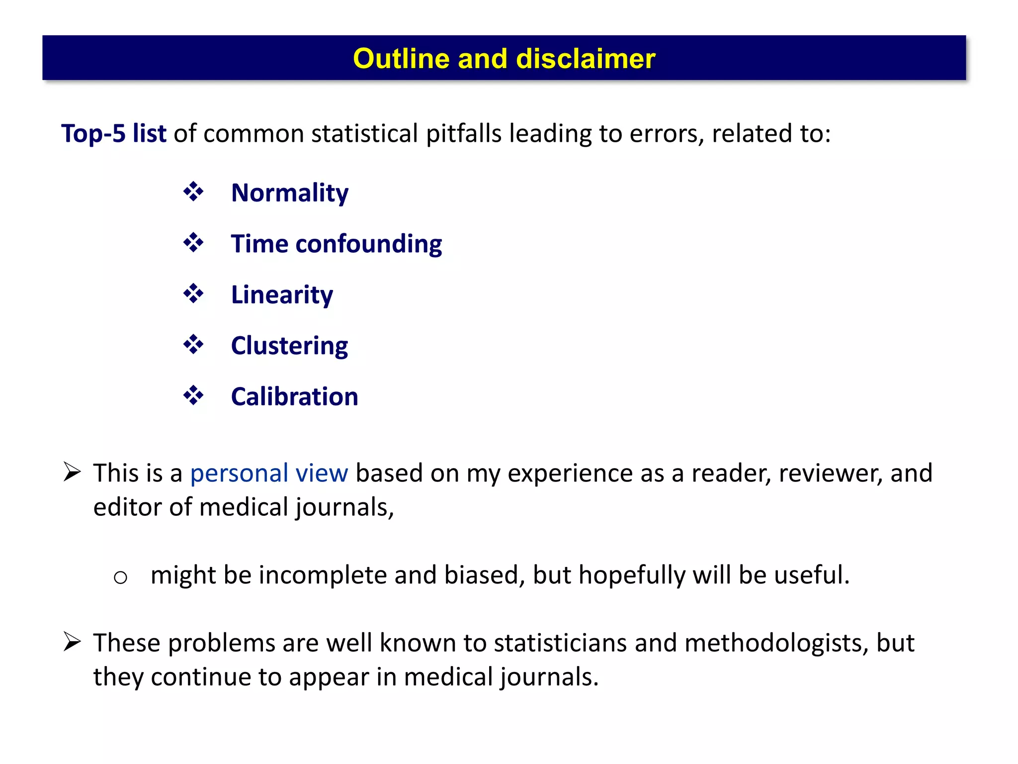
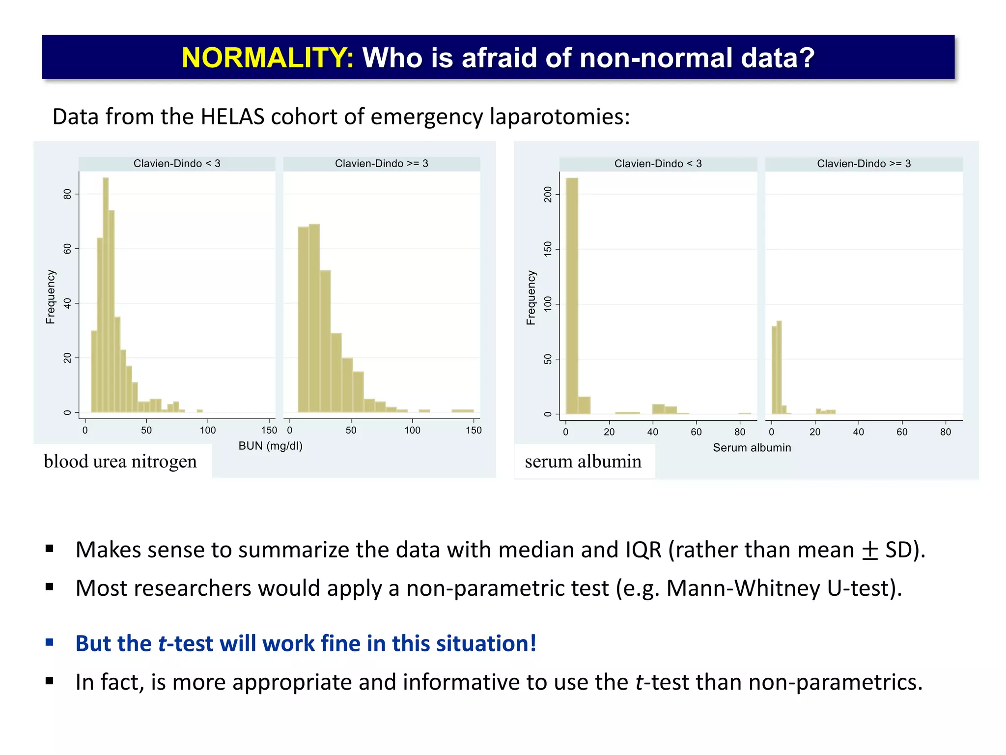


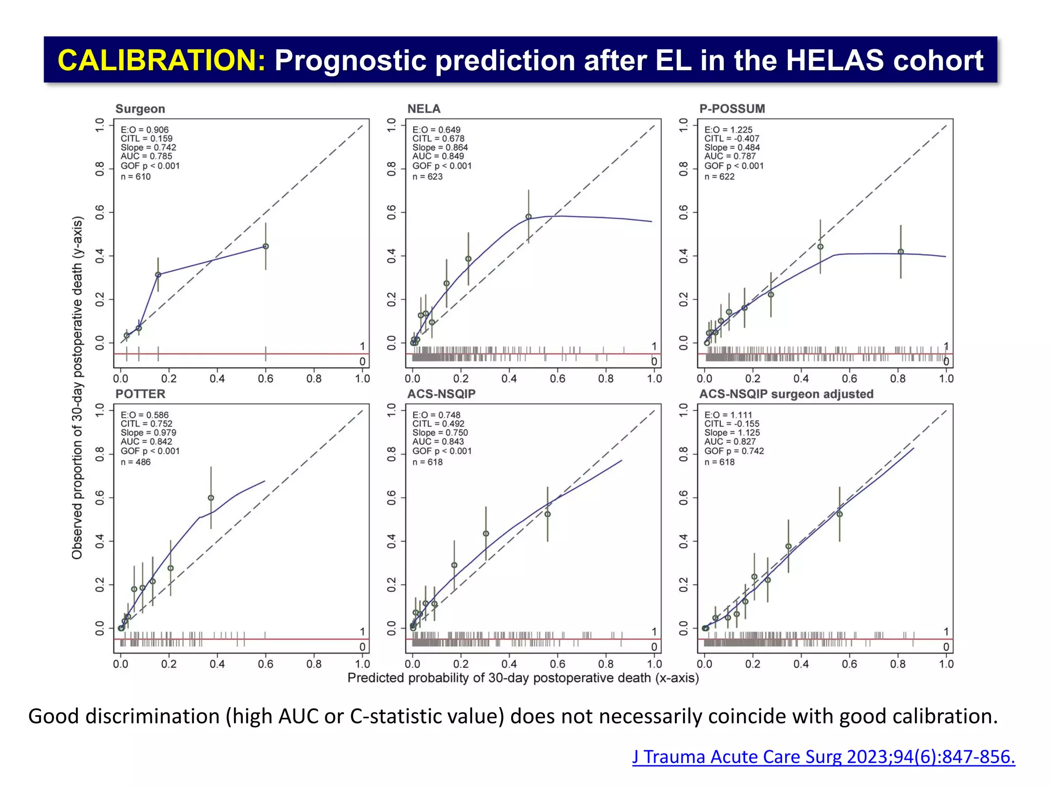

The document outlines five common statistical pitfalls in biomedical research: normality, time confounding, linearity, clustering, and calibration. It emphasizes the misuse of statistical tests and the importance of proper methods like survival analysis for handling censored data, as well as ensuring models account for clustering and avoid overfitting. Recommendations for best practices in statistical analysis are also included, referencing relevant literature for further reading.