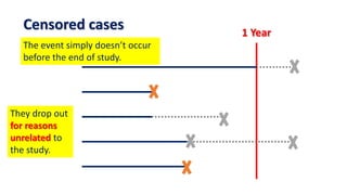
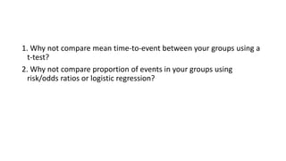
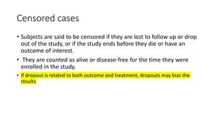
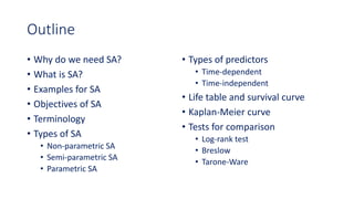
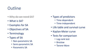
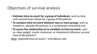
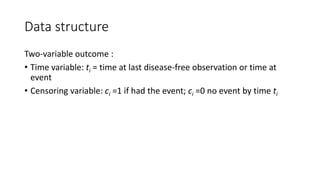
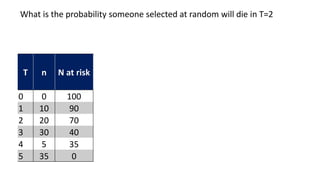
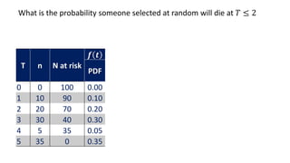
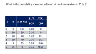
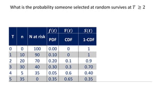
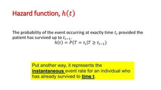
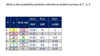
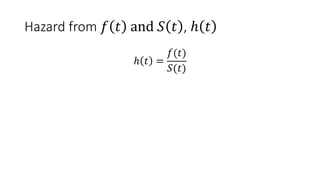
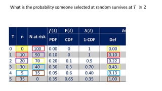
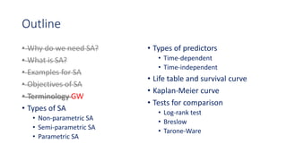
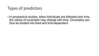
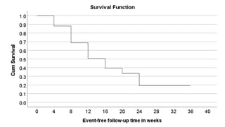
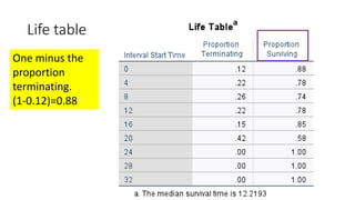
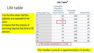
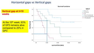
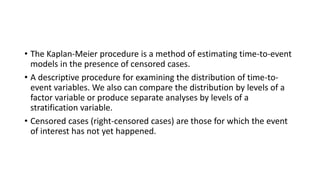
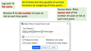
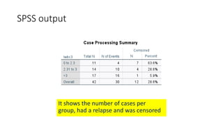
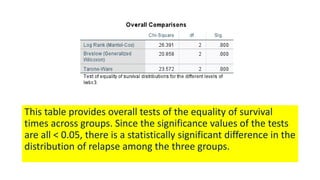
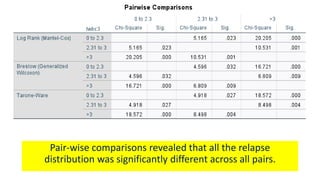
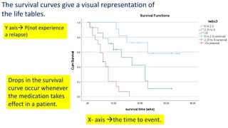
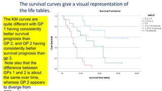
The document introduces survival analysis (SA), a statistical method crucial for analyzing time-to-event data, particularly in the context of clinical trials. It discusses various aspects of SA, including reasons for its need, types of predictors, and methods for comparison, such as the Kaplan-Meier curve and log-rank test. Two clinical trials are highlighted, focusing on lung cancer and ovarian cancer, to exemplify how SA can provide insights into prognosis and treatment outcomes.


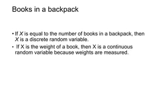


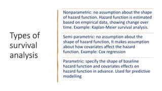


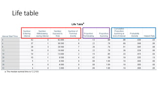
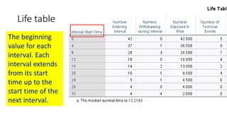
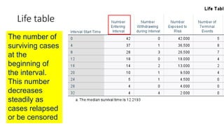

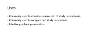
![Life table
An estimate of the
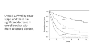
probability of experiencing
the terminal event per time
unit during the interval,
conditional upon surviving
to the start of the interval.
ℎ 𝑡𝑖 =
𝑓(𝑡𝑖)
𝑎𝑣𝑔[𝑆 𝑡𝑖 , 𝑆 𝑡𝑖+1 ]
1st row:
0.03
0.88+1
2
= 0.03
2nd row:
0.48
0.69+0.88
2
= 0.06](https://image.slidesharecdn.com/1-211218104034/85/1-Introduction-to-Survival-analysis-84-320.jpg)
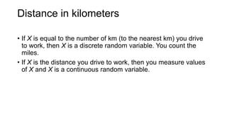
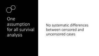
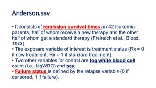
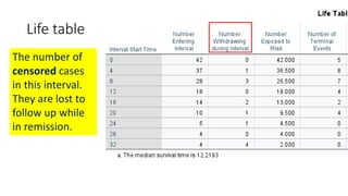
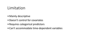
![Life table
An estimate of the
probability of experiencing
the terminal event per time
unit during the interval,
conditional upon surviving
to the start of the interval.
ℎ 𝑡𝑖 =
𝑓(𝑡𝑖)
𝑎𝑣𝑔[𝑆 𝑡𝑖 , 𝑆 𝑡𝑖+1 ]
1st row:
𝟎.𝟎𝟑
𝟎.𝟖𝟖+𝟏
𝟐
= 𝟎. 𝟎𝟑
2nd row:
0.48
0.69+0.88
2
= 0.06
1.00](https://image.slidesharecdn.com/1-211218104034/85/1-Introduction-to-Survival-analysis-85-320.jpg)
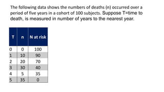
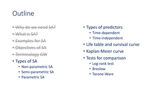
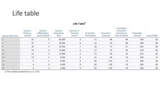
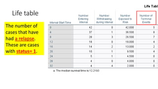
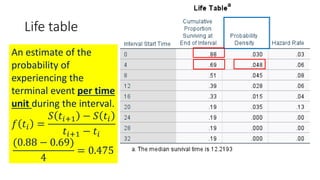
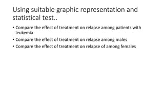
![Life table
An estimate of the
probability of experiencing
the terminal event per time
unit during the interval,
conditional upon surviving
to the start of the interval.
ℎ 𝑡𝑖 =
𝑓(𝑡𝑖)
𝑎𝑣𝑔[𝑆 𝑡𝑖 , 𝑆 𝑡𝑖+1 ]
1st row:
0.03
0.88+1
2
= 0.03
2nd row:
0.48
0.69+0.88
2
= 0.06](https://image.slidesharecdn.com/1-211218104034/85/1-Introduction-to-Survival-analysis-86-320.jpg)


![[DSC Europe 25] Bojan Banjac - AI is always right when it comes to the matter...](https://cdn.slidesharecdn.com/ss_thumbnails/syoxtqierpydwxm5srcb-4-bojan-banjac-ai-is-always-right-when-it-comes-to-the-matters-of-taste-260119101519-694ee7d7-thumbnail.jpg?width=640&height=640&fit=bounds)


![[DSC Europe 25] Borko Kozomora - Optimizing business workflows with advances ...](https://cdn.slidesharecdn.com/ss_thumbnails/hbgekyb0txw0xpo4yfml-borko-kozomora-leading-ai-transformation-260122103838-cc29ee38-thumbnail.jpg?width=640&height=640&fit=bounds)
![[DSC Europe 25] Milovan Jovicic - Beyond AI's Reach: The Enduring Value of Ev...](https://cdn.slidesharecdn.com/ss_thumbnails/pyeij0hurgwq5jugmtnv-2-milovan-jovicic-beyond-ais-reach-the-enduring-value-of-evergreen-design-v2-260120105856-d6ee57e5-thumbnail.jpg?width=640&height=640&fit=bounds)


![[DSC Europe 25] Tali Fulman - Guild Meetings, Then What? Building Data Commun...](https://cdn.slidesharecdn.com/ss_thumbnails/fgohhi33rwmhqdowdj5k-tali-fulman-guild-meetings-then-what-building-data-communities-that-actually-ch-260120105855-528492c3-thumbnail.jpg?width=640&height=640&fit=bounds)
![[DSC Europe 25] Marcos Heidemann - Beyond the Hype: Making AI Coding Assistan...](https://cdn.slidesharecdn.com/ss_thumbnails/eexkhvldrjsopspdjbur-marcos-heidemann-beyond-the-hype-getting-real-value-out-of-ai-assisted-coding-260121115910-7e9d41ec-thumbnail.jpg?width=640&height=640&fit=bounds)

![[DSC Europe 25] Milos Belcevic - Product Professional's Journey to Full-Stack...](https://cdn.slidesharecdn.com/ss_thumbnails/1zovd6fgsycdg4wvgvls-milos-belcevic-product-professionals-journey-to-full-stack-product-developer-260123083019-d993120d-thumbnail.jpg?width=640&height=640&fit=bounds)