A Cox model is a statistical technique used to analyze survival data with several explanatory variables. It allows estimation of the hazard or risk of an event like death for an individual based on prognostic factors. A Cox model expresses the hazard as an exponential function of the explanatory variables. Interpreting a Cox model involves examining the regression coefficients - a positive coefficient means a higher hazard/worse prognosis, while a negative coefficient implies a better prognosis. The model from a study of melanoma patients' survival found age and cancer type increased hazard, while male sex decreased it, and interferon treatment did not significantly impact survival.

1. G A Cox model is a statistical technique for exploring the
relationship between the survival of a patient and several
explanatory variables.
G Survival analysis is concerned with studying the time
between entry to a study and a subsequent event (such as
death).
G A Cox model provides an estimate of the treatment effect
on survival after adjustment for other explanatory variables.
In addition, it allows us to estimate the hazard (or risk) of death
for an individual, given their prognostic variables.
G A Cox model must be fitted using an appropriate computer
program (such as SAS, STATA or SPSS). The final model from a
Cox regression analysis will yield an equation for the hazard
as a function of several explanatory variables.
G Interpreting the Cox model involves examining the coefficients
for each explanatory variable. A positive regression
coefficient for an explanatory variable means that the hazard
is higher, and thus the prognosis worse. Conversely, a negative
regression coefficient implies a better prognosis for patients
with higher values of that variable.
1
What is...? series Second edition Statistics
For further titles in the series, visit:
www.whatisseries.co.uk
Stephen J Walters BSc
MSc PhD CStat Reader in
Medical Statistics, School
of Health and Related
Research (ScHARR),
University of Sheffield
What is a
Cox model?
Supported by sanofi-aventis
Date of preparation: May 2009 NPR09/1005

2. What is the purpose of the
Cox model?
The Cox model is based on a modelling
approach to the analysis of survival data. The
purpose of the model is to simultaneously
explore the effects of several variables on
survival.
The Cox model is a well-recognised
statistical technique for analysing survival
data. When it is used to analyse the survival of
patients in a clinical trial, the model allows us
to isolate the effects of treatment from the
effects of other variables. The model can also
be used, a priori, if it is known that there are
other variables besides treatment that
influence patient survival and these variables
cannot be easily controlled in a clinical trial.
Using the model may improve the estimate of
treatment effect by narrowing the confidence
interval. Survival times now often refer to
the development of a particular symptom or
to relapse after remission of a disease, as well
as to the time to death.
Why are survival times
censored?
A significant feature of survival times is that
the event of interest is very rarely observed in
all subjects. For example, in a study to
compare the survival of patients having
different types of treatment for malignant
melanoma of the skin, although the patients
may be followed up for several years, there
will be some patients who are still alive at the
end of the study. We do not know when these
patients will die, only that they are still alive
at the end of the study; therefore, we do not
know their survival time from the start of
treatment, only that it will be longer than
their time in the study. Such survival times
are termed censored, to indicate that the
period of observation was cut off before the
event of interest occurred.
From a set of observed survival times
(including censored times) in a sample of
individuals, we can estimate the proportion of
the population of such people who would
survive a given length of time under the same
circumstances. This method is called the
product limit or Kaplan–Meier method.
The method allows a table and a graph to be
produced; these are referred to as the life table
and survival curve respectively.
Kaplan–Meier estimate of
the survivor function
The data on ten patients presented in Table 1
refer to the survival time in years following
treatment for malignant melanoma of the
skin.
What is a Cox model?
2
What is
a Cox model?
Date of preparation: May 2009 NPR09/1005
A B C D E F
Survival time Number at Number of Number Proportion Cumulative
(years) risk at start deaths censored surviving until proportion
of study end of interval surviving
0.909 10 1 0 1 – 1/10 = 0.900 0.900
1.112 9 1 0 1 – 1/9 = 0.889 0.800
1.322* 8 0 1 1 – 0/8 = 1.000 0.800
1.328 7 1 0 1 – 1/7 = 0.857 0.686
1.536 6 1 0 1 – 1/6 = 0.833 0.571
2.713 5 1 0 1 – 1/5 = 0.800 0.457
2.741* 4 0 1 1 – 0/4 = 1.000 0.457
2.743 3 1 0 1 – 1/3 = 0.667 0.305
3.524* 2 0 1 1 – 0/2 = 1.000 0.305
4.079* 1 0 1 1 – 0/1 = 1.000 0.305
* Indicates a censored survival time
Table 1. Calculation of Kaplan–Meier estimate of the survivor function

3. 3
What is
a Cox model?
To determine the Kaplan–Meier estimate of
the survivor function for the above example, a
series of time intervals is formed. Each of
these intervals is constructed to be such that
one observed death is contained in the
interval, and the time of this death is taken to
occur at the start of the interval.
Table 1 shows the survival times arranged
in ascending order (column A). Some survival
times are censored (that is, the patient did not
die during the follow-up period) and these are
labelled with an asterisk. The number of
patients who are alive just before 0.909 years
is ten (column B). Since one patient dies at
0.909 years (column D), the probability of
dying by 0.909 years is 1/10 = 0.10. So the
corresponding probability of surviving up to
0.909 years is 1 minus the probability of
dying (column F) or 0.900.
The cumulative probability of surviving up
to 1.112 years, then, is the probability of
surviving at 1.112 years, and surviving
throughout the preceding time interval – that
is, 0.900 x 0.889 = 0.800 (column F). The
third time interval (1.322 years) contains
censored data, so the probability of surviving
in this time interval is 1 or unity, and the
cumulative probability of surviving is
unchanged from the previous interval. This is
the Kaplan–Meier estimate of the survivor
function.
Sometimes the censored survival times
occur at the same time as deaths. The
censored survival time is then taken to occur
immediately after the death time when
calculating the survivor function.
A plot of the Kaplan–Meier estimate of the
survivor function (Figure 1) is a step function,
in which the estimated survival probabilities
are constant between adjacent death times
and only decrease at each death.
An important part of survival analysis is to
produce a plot of the survival curves for each
group of interest.1
However, the comparison
of the survival curves of two groups should be
based on a formal non-parametric statistical
test called the logrank test, and not upon
visual impressions.2
Figure 2 shows the
survival of patients treated for malignant
melanoma: the survival of 338 patients on
interferon treatment was compared with that
of 336 patients in the control group.3
The two
groups of patients appear to have similar
survival and the logrank test supports this
conclusion.
Modelling survival – the Cox
regression model
The logrank test cannot be used to explore
(and adjust for) the effects of several variables,
such as age and disease duration, known to
affect survival. Adjustment for variables that
are known to affect survival may improve the
precision with which we can estimate the
treatment effect.
The regression method introduced by Cox
is used to investigate several variables at a
time.4
It is also known as proportional
hazards regression analysis.
Briefly, the procedure models or regresses
the survival times (or more specifically, the
so-called hazard function) on the explanatory
variables. The actual method is much too
complex for detailed discussion here. This
publication is intended to give an
introduction to the method, and should be of
use in the understanding and interpretation
of the results of such analyses. A more
detailed discussion is given by Machin et al5
and Collett.6
What is a hazard function?
The hazard function is the probability that
an individual will experience an event (for
example, death) within a small time interval,
Date of preparation: May 2009 NPR09/1005
Overall survival (years from surgery)
1.0 –
0.8 –
0.6 –
0.4 –
0.2 –
0.0 –
3 4 50 1 2
Censored
Cumulativeproportionsurviving
Survival function
Figure 1. Kaplan–Meier
estimate of the survival
function

4. given that the individual has survived up to
the beginning of the interval. It can therefore
be interpreted as the risk of dying at time t.
The hazard function – denoted by h(t) –
can be estimated using the following
equation:
number of individuals experiencing
h(t) =
an event in interval beginning at t
(number of individuals surviving at
time t) x (interval width)
What is regression?
If we want to describe the relationship
between the values of two or more variables
we can use a statistical technique called
regression.7
If we have observed the values
of two variables, X (for example, age of
children) and Y (for example, height of
children), we can perform a regression of Y on
X. We are investigating the relationship
between a dependent variable (the height
of children) based on the explanatory
variable (the age of children).
When more than one explanatory (X)
variable needs to be taken into account (for
example, height of the father), the method is
known as multiple regression. Cox’s
method is similar to multiple regression
analysis, except that the dependent (Y)
variable is the hazard function at a given time.
If we have several explanatory (X) variables of
interest (for example, age, sex and treatment
group), then we can express the hazard or risk
of dying at time t as:
h(t) = h0
(t) x exp(bage
.age + bsex
.sex + ...
+ bgroup
.group)
taking natural logarithms of both sides:
ln h(t) = ln h0
(t) x exp(bage
.age + bsex
.sex + ...
+ bgroup
.group)
The quantity h0
(t) is the baseline or
underlying hazard function and corresponds
to the probability of dying (or reaching an
event) when all the explanatory variables are
zero. The baseline hazard function is
analogous to the intercept in ordinary
regression (since exp0
= 1).
The regression coefficients bage
to bgroup
give
the proportional change that can be expected
in the hazard, related to changes in the
explanatory variables. They are estimated by a
complex statistical method called maximum
likelihood,6
using an appropriate computer
program (for example, SAS, SPSS or STATA).
The assumption of a constant relationship
between the dependent variable and the
explanatory variables is called proportional
4
What is
a Cox model?
Date of preparation: May 2009 NPR09/1005
Time from randomisation to death (years)
1.00 –
0.75 –
0.50 –
0.25 –
0.0 –
6 80 2 4
Interferon
Cumulativeproportionsurviving
Control
22
23
0
0
336
338
203
215
97
84
Number at risk
Control
Interferon
Hazard ratio 0.92 (95% CI: 0.74–1.13); p=0.411 (logrank)
Figure 2. Kaplan–Meier
survival curves in
patients receiving
treatment for
malignant melanoma3

5. hazards. This means that the hazard
functions for any two individuals at any
point in time are proportional. In other
words, if an individual has a risk of death at
some initial time point that is twice as high
as that of another individual, then at all later
times the risk of death remains twice as high.
This assumption of proportional hazards
should be tested.6
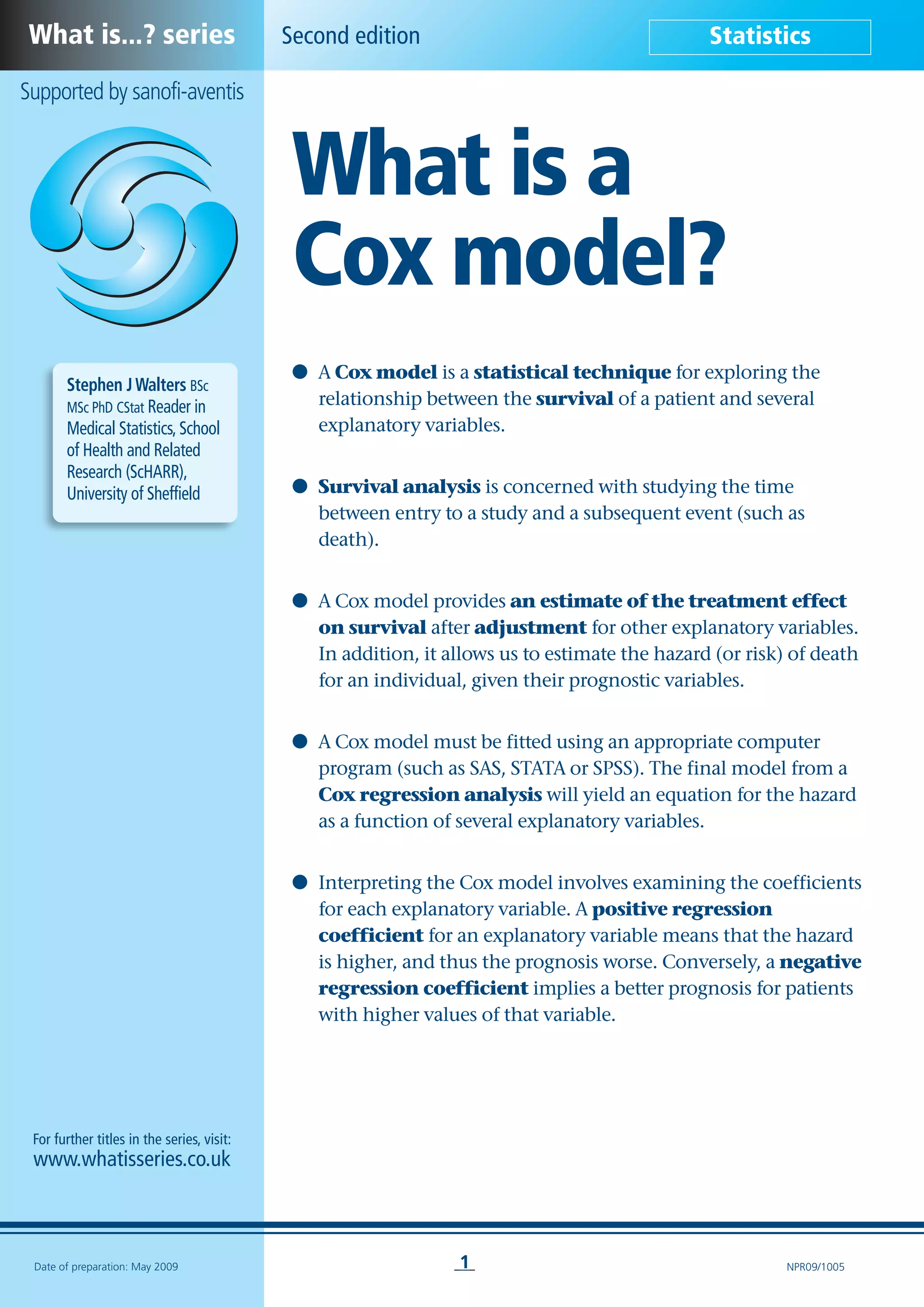
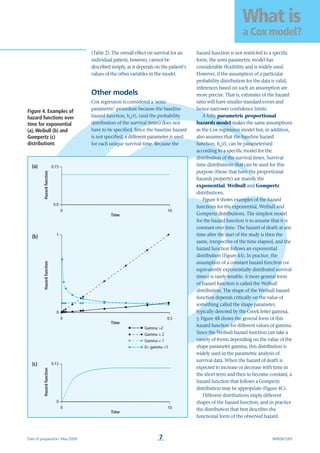
The testing of the proportional hazards
assumption is most straightforward when we
compare two groups with no covariates. The
simplest check is to plot the Kaplan–Meier
survival curves together (Figure 2).3
If they
cross, then the proportional hazards
assumption may be violated. For small data
sets, where there may be a great deal of error
attached to the survival curve, it is possible
for curves to cross, even under the
proportional hazards assumption. A more
sophisticated check is based on what is
known as the complementary log-log plot.
With this method, a plot of the logarithm of
the negative logarithm of the estimated
survivor function against the logarithm of
survival time will yield parallel curves if the
hazards are proportional across the groups
(Figure 3).3
Interpretation of the model
As mentioned above, the Cox model must be
fitted using an appropriate computer
program. The final model from a Cox
regression analysis will yield an equation for
the hazard as a function of several
explanatory variables (including treatment).
So how do we interpret the results? This is
illustrated by the following example.
Cox regression analysis was carried out on
the data from a randomised trial comparing
the effect of low-dose adjuvant interferon alfa-
2a therapy with that of no further treatment
in patients with malignant melanoma at high
risk of recurrence.3,8
Malignant melanoma is a
serious type of skin cancer, characterised by
uncontrolled growth of pigment cells called
melanocytes. Treatments include surgical
removal of the tumour; adjuvant treatment;
chemo- and immunotherapy, and radiation
therapy. In this trial, 674 patients with a
radically resected malignant melanoma (who
were at high risk of disease recurrence) were
randomly assigned to one of two treatment
groups: interferon (3 megaunits of interferon
alfa-2a three times a week until recurrence of
cancer, or for two years – whichever occurred
first) or no further treatment. The primary
5
What is
a Cox model?
Date of preparation: May 2009 NPR09/1005
Randomised
group
Control
Interferon
ln (time)
1 –
0 –
-1 –
-2 –
-3 –
-4 –
-5 –
-6 –
0 1 2-3 -2 -1
ln{–ln[survivalprobability]}
Figure 3. Complementary
log-log plot3

6. 6
aim of this multicentre study was to
determine the effects of interferon on overall
survival. Patients were followed for up to eight
years from randomisation.8
The final Cox model included two
demographic (age and gender) and one
baseline clinical variable (histology) as
independent prognostic factors, plus a
treatment variable (Table 2). An approximate
test of significance for each variable is
obtained by dividing the regression estimate b
by its standard error SE(b), and comparing the
result with the standard normal distribution.
Values of this ratio greater than 1.96 will be
statistically significant at the 5% level. The
Cox model is shown in Table 2.
The first feature to note in such a table is
the sign of the regression coefficients. A
positive sign means that the hazard (risk of
death) is higher, and thus the prognosis
worse, for subjects with higher values of that
variable. Thus, from Table 2, older age and
regionally metastatic cancer histology are
associated with poorer survival, whereas
being male is associated with better survival.
An individual regression coefficient is
interpreted quite easily. Note that patients are
either given interferon (coded as 1) or not
(coded as 0). From Table 2, the estimated
hazard in the interferon group is exp(–0.90) =
0.914 of that of the control group; that is, a
9% decrease in the risk of death after
adjustment for the other explanatory
variables in the model. However, the p-value
of 0.404 is not statistically significant and the
95% confidence interval for the hazard ratio
includes 1, suggesting no difference in
survival. In this study the authors concluded
that there was no significant difference in
overall survival between interferon-treated
patients and those in the control group, even
after adjustment for prognostic factors.8
For explanatory variables that are
continuous (for example, age) the regression
coefficient refers to the increase in log hazard
for an increase of 1 in the value of the
covariate. Thus, the estimated hazard or risk of
death increases by exp(0.004) = 1.004 times if a
patient is a year older, after adjustment for the
effects of the other variables in the model
What is
a Cox model?
Date of preparation: May 2009 NPR09/1005
Variable Regression Standard p-value eb
Hazard 95% CI for
coefficient (b) error SE(b) ratio* hazard ratio
Lower Upper
Age 0.004 0.004 0.359 1.004 0.996 1.012
Sex –0.312 0.110 0.005 0.732 0.590 0.909
(0 = female,
1 = male)
Histology 0.001
Histology (1) –0.033 0.234 0.887 0.967 0.612 1.530
(0 = localised,
1 = LM)
Histology (2) 0.446 0.204 0.029 1.562 1.048 2.330
(0 = localised,
1 = RMD)
Histology (3) 0.569 0.154 0.001 1.766 1.306 2.387
(0 = localised,
1 = RMR)
Group –0.090 0.108 0.404 0.914 0.740 1.129
(0 = control,
1 = interferon)
* Risk of death according to treatment assignment and prognostic variables
CI: confidence interval; LM: locally metastatic; RMD: regionally metastatic at diagnosis; RMR: regionally metastatic at recurrence
Table 2. Cox regression model fitted to the data from the AIM HIGH trial of interferon versus
no further treatment (control) in malignant melanoma (n=674)

7. 7
(Table 2). The overall effect on survival for an
individual patient, however, cannot be
described simply, as it depends on the patient’s
values of the other variables in the model.
Other models
Cox regression is considered a ‘semi-
parametric’ procedure because the baseline
hazard function, h0
(t), (and the probability
distribution of the survival times) does not
have to be specified. Since the baseline hazard
is not specified, a different parameter is used
for each unique survival time. Because the
hazard function is not restricted to a specific
form, the semi-parametric model has
considerable flexibility and is widely used.
However, if the assumption of a particular
probability distribution for the data is valid,
inferences based on such an assumption are
more precise. That is, estimates of the hazard
ratio will have smaller standard errors and
hence narrower confidence limits.
A fully parametric proportional
hazards model makes the same assumptions
as the Cox regression model but, in addition,
also assumes that the baseline hazard
function, h0
(t), can be parameterised
according to a specific model for the
distribution of the survival times. Survival
time distributions that can be used for this
purpose (those that have the proportional
hazards property) are mainly the
exponential, Weibull and Gompertz
distributions.
Figure 4 shows examples of the hazard
functions for the exponential, Weibull and
Gompertz distributions. The simplest model
for the hazard function is to assume that it is
constant over time. The hazard of death at any
time after the start of the study is then the
same, irrespective of the time elapsed, and the
hazard function follows an exponential
distribution (Figure 4A). In practice, the
assumption of a constant hazard function (or
equivalently exponentially distributed survival
times) is rarely tenable. A more general form
of hazard function is called the Weibull
distribution. The shape of the Weibull hazard
function depends critically on the value of
something called the shape parameter,
typically denoted by the Greek letter gamma,
γ. Figure 4B shows the general form of this
hazard function for different values of gamma.
Since the Weibull hazard function can take a
variety of forms depending on the value of the
shape parameter gamma, this distribution is
widely used in the parametric analysis of
survival data. When the hazard of death is
expected to increase or decrease with time in
the short term and then to become constant, a
hazard function that follows a Gompertz
distribution may be appropriate (Figure 4C).
Different distributions imply different
shapes of the hazard function, and in practice
the distribution that best describes the
functional form of the observed hazard
What is
a Cox model?
Date of preparation: May 2009 NPR09/1005
Time
0.15 –
0.0 –
100
Hazardfunction
Time
0.12 –
0 –
100
Hazardfunction
Gamma >2
Gamma = 2
Gamma = 1
0< gamma <1
1 –
0 –
Hazardfunction
Time
0.50
Figure 4. Examples of
hazard functions over
time for exponential
(a),Weibull (b) and
Gompertz (c)
distributions
(a)
(b)
(c)

8. Supported by sanofi-aventis
What is
a Cox model?
Published by Hayward Medical
Communications, a division of
Hayward Group Ltd.
Copyright © 2009 Hayward
Group Ltd.
All rights reserved.
8
What is...? series
First edition published 2001
Author: Stephen J Walters
This publication, along with
the others in the series, is
available on the internet at
www.whatisseries.co.uk
The data, opinions and statements
appearing in the article(s) herein
are those of the contributor(s)
concerned.Accordingly, the
sponsor and publisher, and their
respective employees, officers
and agents, accept no liability
for the consequences of any such
inaccurate or misleading data,
opinion or statement.
Date of preparation: May 2009 NPR09/1005
function is chosen.6
Fitting three parametric
proportional hazard models, assuming
exponential, Weibull and Gompertz baseline
hazards, to the malignant melanoma trial
data produced similar regression coefficients
to the standard Cox model in Table 2.
A family of fully parametric models that
accommodate, directly, the multiplicative
effects of explanatory variables on survival
times, and hence do not have to rely on
proportional hazards, are called accelerated
failure time models. These models are too
complex for a discussion here, and a more
detailed discussion is given by Collett.6
References
1. Freeman JV, Walters SJ, Campbell MJ. How to display data.
Oxford: Blackwell BMJ Books, 2008.
2. Altman DG. Practical Statistics for Medical Research. London:
Chapman & Hall/CRC, 1991: 365–396.
3. Dixon S, Walters SJ, Turner L, Hancock BW. Quality of life and
cost-effectiveness of interferon-alpha in malignant melanoma:
results from randomised trial. Br J Cancer 2006; 94: 492–498.
4. Cox DR. Regression models and life tables. J Roy Statist Soc B
1972; 34: 187–220.
5. Machin D, Cheung YB, Parmar M. Survival Analysis: A Practical
Approach, 2nd edn. Chichester: Wiley, 2006.
6. Collett D. Modelling Survival Data in Medical Research, 2nd edn.
London: Chapman & Hall/CRC, 2003.
7. Campbell MJ, Machin D, Walters SJ. Medical Statistics: A text
book for the health sciences, 4th edn. Chichester: Wiley, 2007.
8. Hancock BW, Wheatley K, Harris S et al. Adjuvant interferon in
high-risk melanoma: the AIM HIGH Study – United Kingdom
Coordinating Committee on Cancer Research randomized study
of adjuvant low-dose extended-duration interferon Alfa-2a in
high-risk resected malignant melanoma. J Clin Oncol 2004; 22:
53–61.
Further reading
Chapter 13 of Altman2
provides a good introduction to survival
analysis, the logrank test and the Cox regression model. A more
detailed technical discussion of survival analysis and Cox
regression is given by Machin et al and Collett.5,6
Box 1. Glossary of terms
Confidence interval (CI). A range of values,
calculated from the sample of observations
that are believed, with a particular probability,
to contain the true parameter value. A 95%
confidence interval implies that if the
estimation process were repeated again and
again, then 95% of the calculated intervals
would be expected to contain the true
parameter value. Note that the stated
probability level refers to the properties of the
interval and not to the parameter itself.
ex
or exp(x). The exponential function,
denoting the inverse procedure to that of
taking logarithms.
Logrank test. A method for comparing the
survival times of two or more groups of
subjects. It involves the calculation of observed
and expected frequencies of failures in
separate time intervals. The relevant test
statistic is a comparison of the observed
number of deaths occurring at each particular
point with the number to be expected if the
survival experience of the two groups is
the same.
Logarithms. Logarithms are mainly used in
statistics to transform a set of observations to
values with a more convenient distribution.
The natural logarithm (loge
x or ln x) of a
quantity x is the value such that x = ey
. Here e
is the constant 2.718281… The log of 1 is 0
and the log of 0 is minus infinity. Log
transformation can only be used for data
where all x values are positive.
SE or se. The standard error of a sample
mean or some other estimated statistics (for
example, regression coefficient). It is the
measure of the uncertainty of such an
estimate and it is used to derive a confidence
interval for the population value. The notation
SE(b) means the ‘standard error of b’.
p. The probability value, or significance level,
from a hypothesis test. p is the probability of
the data (or some other more extreme data)
arising by chance when the null hypothesis
is true.