Downloaded 65 times
![PhUSE 2008
3
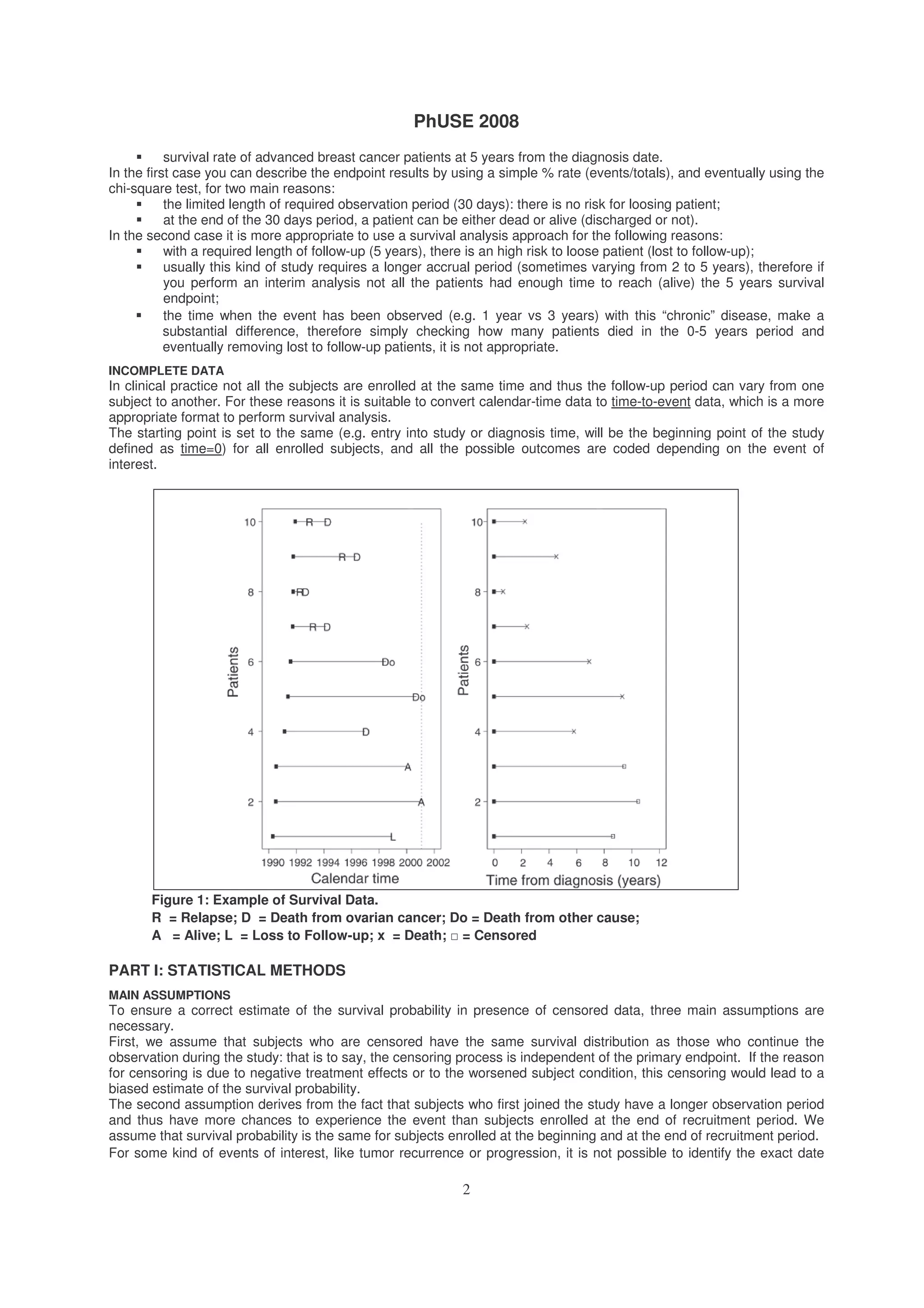
when the event happens, because the only information we would have is the event happened between two subsequent
examinations. In this case we need to assume that the event happens at the time it is detected, otherwise we would
obtain a biased estimate of the survival times.
CALCULATION OF SURVIVAL PROBABILITY: THE KAPLAN-MEIER METHOD
Survival data are described in terms of two probabilities: survival and hazard.
The first one is the probability for an individual to survive from the starting time until a specified future time t.
To estimate the proportion of subjects surviving at a given time point, and hence the survival probability to that time for
the generic population from which the sample is extracted, the Kaplan-Meier method [1][2][3][4][5][6][7], also called
product-limit estimator, is commonly used, which allows to deal with censored information.
The simple idea underlying this method is that to survive to k intervals from the start of the study, it is necessary to
survive to each one of the previous intervals, and then also to the k
th
one. This principle allows working with conditional
and cumulative probabilities.
The conditional survival probability for the generic time interval (on the condition that the subject was survivor at the
beginning of the interval and then to all the previous) is given by:
i
ii
i
r
dr
p
−
=
where r is the number alive and at risk at the beginning of the i
th
interval, and d the number of failures during the same
interval. Observations censored at any given time influence the number at risk at the start of the subsequent time
interval.
Survival at any time point is calculated as product of the conditional probabilities of surviving each previous time
interval.
∏≤
−=
ti i
i
r
d
tS )1()(
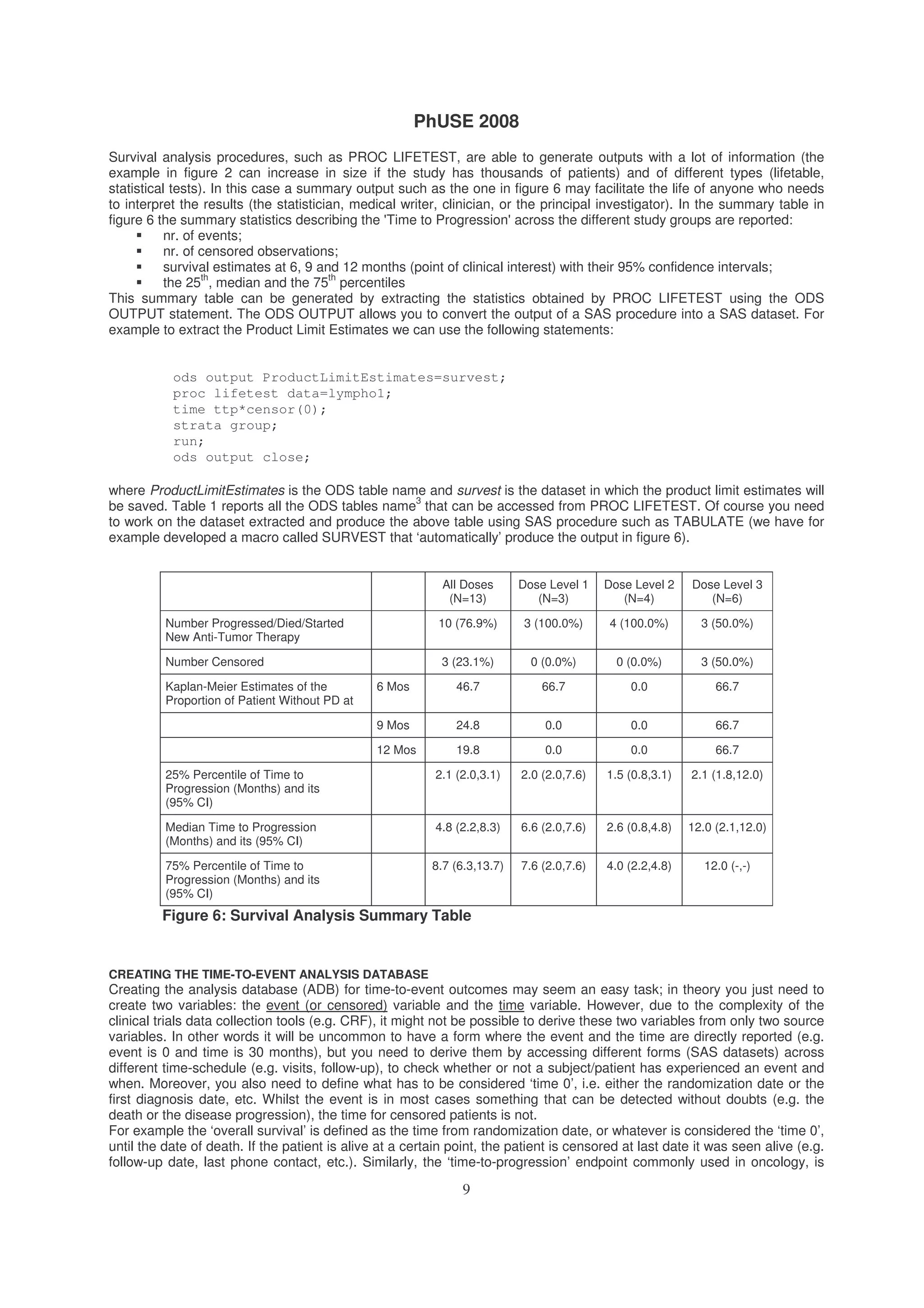
Figure 2 is an example of survival probability calculation, derived from a SAS output referred to time to progression
data (time expressed in weeks).](https://image.slidesharecdn.com/st03-140317102040-phpapp02/75/A-gentle-introduction-to-survival-analysis-3-2048.jpg)
![PhUSE 2008
4
Figure 2: Survival probabilities Calculation
At week 0, all enrolled subjects (17) are alive and at risk to experience the event of interest (progression). Survival
probability is thus set to 1
1
.
At week 6, a censoring occurs (but number failed is still 0): it does not modify the survival and failure probabilities, but
the number of subjects at risk for the subsequent interval decreases by one (number left = 16).
At week 10, two events occur, thus all the statistics are modified: the number failed increases by two, while the number
left still at risk for the subsequent interval reduces to 14. Survival probability for the interval [time 0 to time 10] is then
equal to (16-2)/16=0.8750.
A new event occurs at week 16, together with two censored observations; the survival probability for the interval [week
10 to week 16] is equal to (14-1)/14=0.9286. To calculate the cumulative probability for a subject to survive from the
start of the study until the week 16 it is now necessary to cumulate the survival probabilities for each time interval.
Cumulative survival probability until time 16 is computed as 0.9286 x 0.8750 = 0.8125.
At week 17 a new event occurs: the survival probability for the time interval [week 16 to week 17] is computed as (11-
1)/11=0.9091.
Cumulating all the previous single probabilities, we can easily obtain the probability for a subject enrolled at the
beginning of the study to survive without experiencing the event until week 17: 0.9091 x 0.9286 x 0.8750 = 0.7387.
The same process can be followed until week 44 when no more events are available and the survival probability can’t
be modified anymore.
SURVIVAL PROBABILITIES CALCULATION: THE LIFETABLE METHOD
In some situations it is not possible to know or to record the exact time when the event occurs; the only available
information is that the event occurred in a certain time interval. In this case the survival probability cannot be updated
every time an event happens, but once in a fixed time unit: the derived survival curve and probability are called life-
table or actuarial estimates.
With this method, the whole period of observation is divided into a series of time intervals, where the basic assumption
is that censorings are uniformly distributed in each interval, so that the average number of subjects at risk during each
interval is given by:
2
' j
jj
c
nn −=
Where n’j is the number of subjects alive and at risk at the beginning of the time interval j and cj is the number of
censored observations in the same interval.
As previously seen with the Kaplan-Meier method, the cumulative probability to survive until the time t is given by the
product of the probabilities to survive to each previous time interval and also to the last one including t.
∏≤
−=
tj j
j
i
n
d
tS )1()( '
dj is the number of deaths or events observed in the time interval j.
THE GRAPHICAL REPRESENTATION
Survival probability can be plotted against survival time, obtaining a survival curve: the survival curve is a non-
increasing function with a step corresponding at each time when an event is observed; the step is used since the
estimated survival curve remains at a plateau between successive patient event time and it drops instantaneously at
each time of event to a new level. Times when a censoring happens are usually indicated with a small circle or a short
vertical line. The plot will never reach ‘0’ if the patient with longest observed time has in fact died. Were such a patient
still alive then the curve would have a plateau commencing at the time of the last event and continuing until the
censored observed time of this longest ‘surviving’ patient.
In certain circumstances a graph of 1-S(t), rather than S(t), is plotted against time to give the cumulative ‘event’ curve.
From the graphical representation of a survival curve it is possible to extract relevant summary statistics, mainly the
median survival time and the survival probability at a certain time point.
The median survival time is defined as the time point when half of the subjects have experienced the event of interest,
and can be easily determined by drawing a line (the red line in Figure 3) starting from the value 0.5 on the vertical axis
until you reach the survival curve, and then from the curve till the horizontal time axis. The exact value of the median
1
It can be also expressed as % (see figure 6)](https://image.slidesharecdn.com/st03-140317102040-phpapp02/75/A-gentle-introduction-to-survival-analysis-4-2048.jpg)
![PhUSE 2008
5
survival time can be calculated with a proportion involving the length of the axis and the maximum follow-up time
observed. Similarly you can extract the median from the estimates (figure 2) by searching for the first estimate below
0.50; in the case the 0.50 (or below) is not reached, we say “the median of survival has been not yet reached”. This
latter situation, can happen when cohorts with low event rate or in the case of early (interim) analysis. Again in the
same way you can extract other percentiles of interest, typically the 25% and the 75%, by searching the point in which
the curve reach the point of interest (e.g. .25 and .75).
The survival probability at a certain time point (e.g. 20 months, Figure 3) can be calculated in a similar way: as shown
by the blue line in Figure 3, it is necessary to draw a line from the chosen point of the horizontal time axis to the
survival curve, and then until the vertical survival probability axis. Once again, the exact probability can be deduced
using a proportion involving the length of the vertical axis and the maximum value of the survival probability.
It is difficult to judge precisely when the right-hand tail of the survival curve becomes unreliable. However, as rule of
thumb, the curve can be particularly unreliable when the number of patients remaining at risk is less than 15 or more in
general less than 5%.
Another important statistic you may be required to provide, is the median of follow-up. The median of follow-up is an
indicator of how ‘mature’ are your data by giving an estimate of the length of the observation period (e.g. how many
months on ‘average’ the patients have been followed since they have been enrolled). To calculate the median of follow-
up we can use survival analysis approach by censoring patients who experienced the event. The reason for that is
because you don’t know how long you could follow a patient if this did not experience the event.
Figure 3: Survival Curve with Censored Observations: Median Survival (red line) Time and
Survival Probability at a Fixed Time Point (blue line).
COMPARING SURVIVAL CURVES
An interesting issue in the clinical practice is the comparison of the survival functions of two (or more) groups of
subjects.
Classical statistical methods such as T-test or Chi-square Test are not appropriate to compare the proportion of
survivors for the reasons described before.
Alternatively, one could compare the proportions surviving at one or more pre-specified time points, but this approach
ignores the total survival experience of the groups during the whole follow-up period. Moreover, the time points are
arbitrary chosen.
The most common method used to compare survival curves is then a statistical hypothesis test called log-rank test [8],
which takes the whole follow-up period into account and does not require any assumption about the distribution of the
survival function, which is rarely normally distributed and is often skewed because it often comprises many early events
and only a few late ones.
The null hypothesis for the log-rank test is that there is no difference between the survivals of two or more populations
that are being compared (i.e. the probability of the event of interest occurring at any time point is the same for each
The median survival
is about 63 months
At 60 months the %
survival is about .58](https://image.slidesharecdn.com/st03-140317102040-phpapp02/75/A-gentle-introduction-to-survival-analysis-5-2048.jpg)
![PhUSE 2008
6
population).
The comparison is based on the difference between the observed number of events in each group and the expected
number of events in case of non-difference between the two groups.
−
=−
g g
gg
rank
E
EO 2
log
2
)(
χ
where O is the number of observed events in each group g, and E is the total number of expected events in each group
g. O and E are calculated for each time when an event happens; if a survival time is censored, then the subject is
considered to be at risk during the interval of censoring, but not anymore for the subsequent intervals.
The test statistic is then compared with a
2
with g-1 degrees of freedom.
The log-rank test assigns equal weight to each event at whatever time it occurs.
If researchers believe that differences between certain parts of the survival curves being compared are of greater
interest than others, then different weights can be assigned to the deaths, depending on the time when they happen.
For example, if it were known that a new treatment is helpful to avoid early mortality, then it would be useful to compare
the first part of the survival curves, without paying too much attention to the subsequent time intervals.
The best way to achieve this aim is to construct a statistical test using as weights the number of patients at risk at each
time point: this test is a variant of the log-rank test and it is known as Gehan or generalized Wilcoxon or Breslow test
and can be calculated as follows:
−
=
tg gtt
gtgtt
G
ER
EOR
,
2
2
2
)(
χ
where R is the number of patients at risk in each group and for each time point.
Note that these are tests of significance, and do not provide an estimate of the size of the differences in survival
probabilities between the groups.
COX REGRESSION MODEL AND HAZARD RATIO
While with previous described methods, either the Kaplan-Meier or the Life-Tables method, the survival data are
analyzed using an univariate approach.
To approach survival analysis in a multivariate way, the Cox model is used [9][10]. The Cox model a semi-parametric
regression model used to test the effect of a set of covariates X1, X2, …, Xn on the time-to-event variable; the model for
the hazard function is the following:
{ }nn xxxtth βββλ +++⋅= ...exp)()( 2211
where h(t) represents the hazard function and (t) is an unspecified initial hazard function.
The hazard is a function of time and represents the instantaneous probability that the event of interest will occur at a
specified time t given that it has not occurred prior to time t.
Hazard is defined as follows:
t
tNtentsobservedev
t ∆→∆
)(/)(
lim
0
Where N is the number of subjects at risk at the beginning of the time interval.
The Cox model (that, as with the Kaplan-Meier method, also adjusts for censored data) can include one or more
numeric covariates (which can be also time-dependent) and does not make any assumption on the distribution of the
event times.
The main assumption of the Cox proportional hazard regression model is that the hazard ratio between the treatment
groups remains constant over time, even if, as it is reasonable to assume, the hazard rate does change over time.
D. R. Cox, after whom the model is named, developed a method to estimate the coefficients i based on a maximal
partial likelihood, which is a modification of the maximum likelihood method.
Chi-square tests are performed to evaluate the null hypothesis of non-significance of the i parameters. A positive
parameter estimate indicates that the hazard increases with increasing values of the covariate, while a negative
estimate shows that the hazard decreases with increasing values of the covariate
The magnitude of the effect of a specific covariate on the event time is often expressed as hazard ratio [11]: this is an
estimate of the relative survival experience of two groups and can be calculated as](https://image.slidesharecdn.com/st03-140317102040-phpapp02/75/A-gentle-introduction-to-survival-analysis-6-2048.jpg)
![PhUSE 2008
7
cc
ee
EO
EO
/
/
If the hazard ratio indicates a beneficial effect of the treatment on study, this implies that the time to the observed
endpoint was modified by treatment.
The hazard ratio derived from the Cox regression model does not translate directly into information about the duration
of time until the event occurs, but it can be converted, anyway, in terms of absolute risk reduction, showing the
difference between the risk in the control group (set to 1) and the risk in the treated group (that is hazard ratio itself).
Absolute risk reduction is defined thus as 1 – HR, and can be expressed either as a probability or as a percentage.
PART II: STATISTICAL PROGRAMMING ASPECTS
ILLUSTRATIVE STUDY: OVARIAN CANCER STUDY
This data set refers to a multicenter, phase III, randomized clinical trial involving women with epithelial ovarian
carcinoma randomized to either receive a more (Lymphadenectomy) or less (No Lymphadenectomy or Surgery Only)
invasive surgery; the main end-points of the study included progression-free and overall survival [12].
427 eligible patients were enrolled: 211 were randomly assigned to the surgery only arm, while 216 to the
lymphadenectomy arm.
After a median follow-up of 68.4 months, tumor recurrence was observed in 292 patients (153 in the surgery alone arm,
and 139 in the lymphadenectomy arm).
Figure 4 shows the survival curve for these data.
Figure 4: Result of survival analysis for the ovarian cancer trial.
The Number of patients still at risk at each time point for the treated and control groups are shown below the horizontal
axis; you can also decide to add the number of events occurred in each interval (e.g. between year 1 and year 2).
The unadjusted hazard ratio for the risk of a first event in the lymphadenectomy group, as compared with the surgery
alone group, was 0.76 (95% CI 0.60 to 0.96), meaning that the risk of a recurrence of disease is lower in the patients
treated with lymphadenectomy if compared with the control group.
The absolute gain in survival for the treated group is equal to (1-0.76)*100=24%. This difference in survival probabilities
of the two compared groups is statistically significant (P=0.022 using the log-rank test).
Median progression-free survival was 22.4 months for patients in the control arm and 27.4 months for patients in the
systematic lymphadenectomy arm, confirming the improvement in survival for the patients treated with additional
lymphadenectomy.
These results can be obtained using Proc LIFETEST. Proc LIFETEST computes non-parametric estimates of the
survival distribution and rank tests for associations of the response variable with other variables. The survival estimates](https://image.slidesharecdn.com/st03-140317102040-phpapp02/75/A-gentle-introduction-to-survival-analysis-7-2048.jpg)
![PhUSE 2008
8
are computed within defined strata levels and the rank tests are pooled over the strata and are therefore adjusted for
strata differences. Additionally, statistics testing of homogeneity of the strata are computed.
proc lifetest data=lympho1 plot=(s);
time ttp*censor(0);
strata group;
run;
The PLOTS statement displays the survival curve for the data considered. The statement TIME requests the variable
for time to progression (ttp) and the variable indicating censoring (censor); the value between round brackets (0) is the
one associated to censored observations, STRATA is the variable for the groups to be compared (group). By default
the estimates are calculated using the Kaplan-Meier method.
The same code can be used for calculating median of follow-up by changing the censoring indicator from ‘0’ to ‘1’ if ‘1’
indicates the occurrence of the event of interest.
Cox proportional hazards analysis was performed to adjust the treatment comparison for baseline characteristics:
results are shown in Figure 5.
When histologic grade and residual disease were taken into account, the adjusted hazard ratio for occurrence of first
event was almost unchanged (0.75 [95% CI = 0.59 to 0.94]), confirming that the 25% improvement in survival for
patients treated with additional lymphadenectomy depends mostly on treatment received. These results can be
obtained using PROC PHREG.
Figure 5: Multivariable Cox proportional hazards analysis for PFS
Proc PHREG procedure performs regression analysis of survival data based on the Cox proportional hazards model.
Adopting a partial likelihood function, Cox regression eliminates the unknown baseline hazard and accounts for
censoring survival times. It also allows the use time dependent explanatory variable, which is one whose values for any
given individual can change over time
proc phreg data=lympho2;
model ttp*censor(0)=group grade residual;
run;
The statement MODEL requests to specify the dependent (ttp, censor) and independent (group, grade, residual)
variables to fit the regression model; the Hazard ratios are automatically calculated.
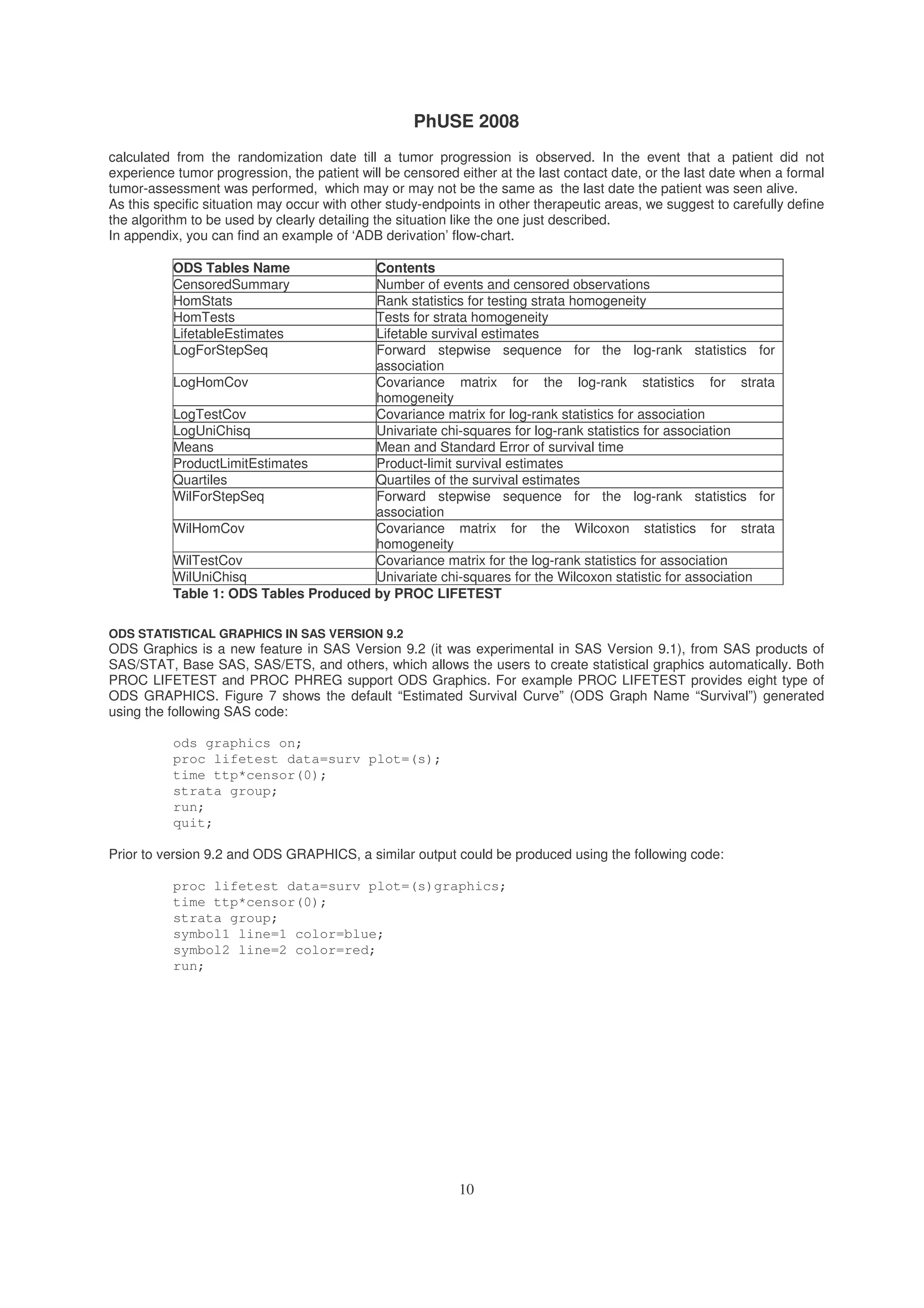
EXTRACTING SUMMARY STATISTICS
3
If you want to know which ODS table should be used to access a portion of the output of the SAS procedure you are
using, you can simply use the statement ODS TRACE ON before using the procedure and use the statement ODS
TRACE OFF when you want to stop ODS tracing. The name of the ODS tables used/generated by the SAS procedure,
will be reported in the LOG file.](https://image.slidesharecdn.com/st03-140317102040-phpapp02/75/A-gentle-introduction-to-survival-analysis-8-2048.jpg)
![PhUSE 2008
11
Figure 7: Graphical Survival Plot with ODS Graphics
META-ANALYSIS OF TIME-TO-EVENT DATA
Meta-analyses (MA) that combine the results of related randomised controlled trials have become a common and
widely accepted tool in the evaluation of health care interventions. Regulatory agencies such as the FDA have started
considering it as key supporting evidence. Systematic reviews use explicit, objective and prospectively-defined
methods to collect, critically evaluate and synthesize studies, making them less biased and more reproducible than
traditional reviews. A systematic review may, or may not, include a meta-analysis (MA): a statistical pooling of the
results from individual studies to obtain a single overall estimate of treatment effect. Today there are well validated
method to perform also meta-analysis of time-to-event data [13] [14].
ADDITIONAL TECHNICAL REFERENCES
Apart the methodological references you can find in the ‘References’ section, we want to suggest to have a look at the
following articles presented at various SAS users congress:
Smith T. Smith B. Kaplan Meier and Cox Proportional Hazard Modelling: Hands on Survival Analysis. WUSS.
2004
Yeh S. ODS and Statistical Graphics. Paper PR02. NESUG17. 2004
Zhou JC. Enhancement of Survival Graphs. Paper 239-28. SUGI28
Xu W. Wang WWB %KMPLOT – An enhancement of SAS PROC LIFETEST. Paper SP06. PharmaSUG.
2005
Smoak C. Survival (Kaplan-Meier) Curves made Easy. Paper TT07. PharmaSUG. 2006
Gharibvand L. Fernandez G. Advanced Statistical and Graphics features of SAS PHREG. Paper 375. SAS
Global Forum. 2008
CONCLUSIONS
Survival analysis is a method of analyzing time to event data when such data are exposed to a censoring process,
whereby subjects finish a clinical trial without having experienced an event. Other statistical methods cannot
adequately take into account the censoring process since they do not adjust for the 'risk' population decreasing as the
subject leaves the trial. Statistical procedures such as Proc LIFETEST and Proc PHREG are the tools with which
the statistician/programmer has to work with within the SAS system. Statistical programmers require a fundamental
understanding of the methodology so that they are able to understand, and eventually check, the results that they are
without doubts responsible for.
REFERENCES
1. Kaplan EL. Meier P. Nonparametric estimation from incomplete observations. J Am Statistics Association 1958;
53:457-81
2. Bewick V., Cheek L., Ball J. Statistics review 12: survival analysis. Crit Care 2004 Oct;8(5):389-94. Epub 2004 Sep
6.
3. Douglas G Altman, J Martin Bland. Statistics Notes: Time to event (survival) data. BMJ 1998; 317; 468-469
4. J Martin Bland , Douglas G Altman. Statistics Notes: Survival probabilities (the Kaplan-Meier method). BMJ 1998;](https://image.slidesharecdn.com/st03-140317102040-phpapp02/75/A-gentle-introduction-to-survival-analysis-11-2048.jpg)

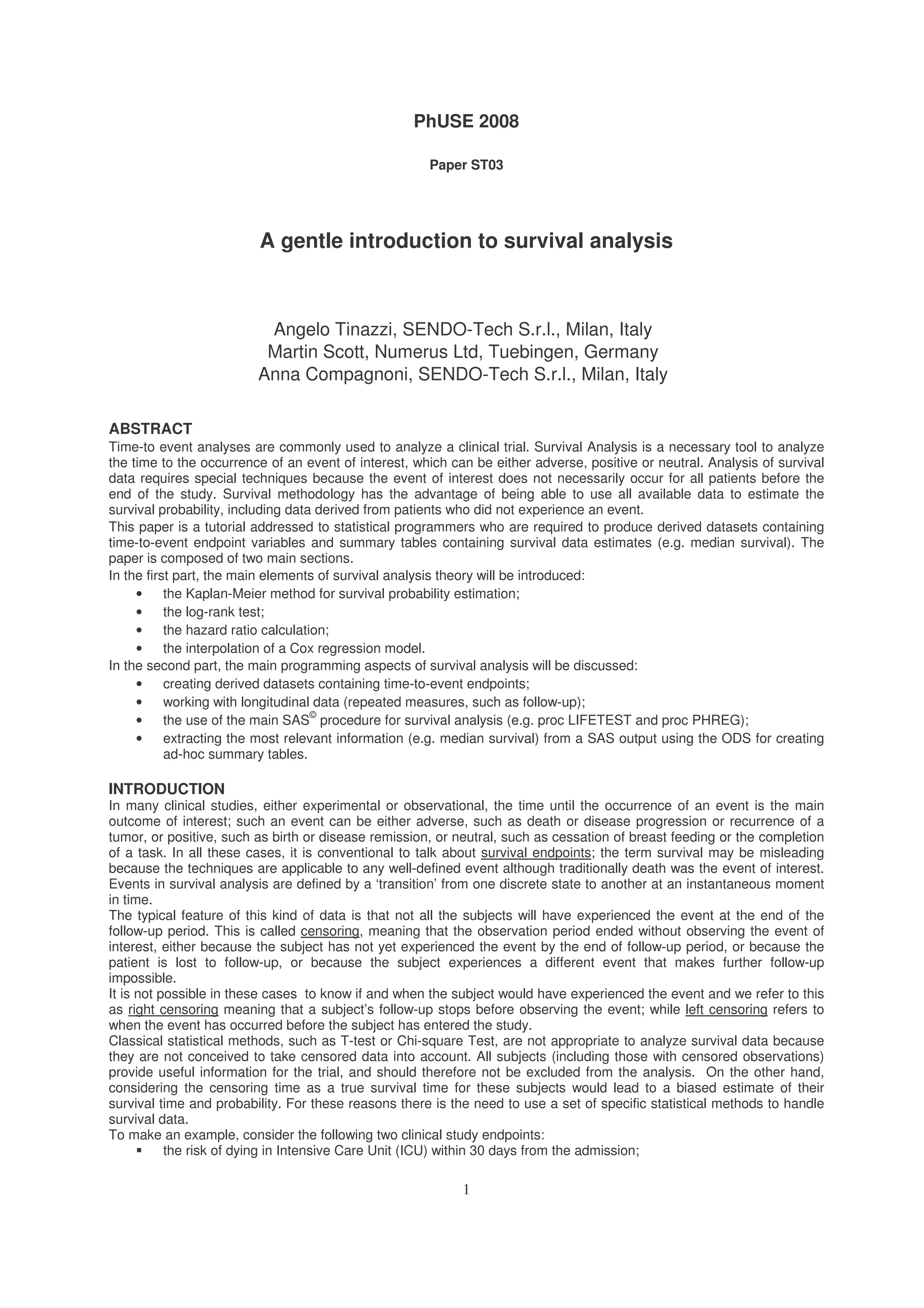
This document provides an introduction to survival analysis techniques for statistical programmers. It discusses key concepts in survival analysis including censoring, the Kaplan-Meier method for estimating survival probabilities, and assumptions of survival models. Programming aspects like creating time-to-event datasets and using SAS procedures for survival analysis are also covered.