This document discusses survival analysis techniques. It begins with an overview of survival, censoring, and the need for survival analysis when not all patients have died or had the event of interest. It then describes the key techniques of life tables/actuarial analysis and the Kaplan-Meier method. Life tables involve constructing a hypothetical cohort and estimating survival at different ages based on mortality rates. The Kaplan-Meier method is commonly used to illustrate survival curves and gives partial credit to censored observations. A modified life table is also presented to analyze survival outcomes in different treatment groups.

1. Survival analysis
Dr HAR ASHISH JINDAL
JR

2. Contents
•
•
•
•
•
•
•
•
•
Survival
Need for survival analysis
Survival analysis
Life table/ Actuarial
Kaplan Meier product limit method
Log rank test
Mantel Hanzel method
Cox proportional hazard model
Take home message

3. Survival
• It is the probability of remaining alive for a
specific length of time.
• point of interest : prognosis of disease e.g.
– 5 year survival
e.g. 5 year survival for AML is 0.19, indicate 19% of
patients with AML will survive for 5 years after
diagnosis

4. Survival
• In simple terms survival (S) is mathematically
given by the formula;
S = A-D/A
A = number of newly diagnosed patients under
observation
D= number of deaths observed in a specified period

5. e.g For 2 year survival:
S= A-D/A= 6-1/6 =5/6 = .83=83%

6. e.g For 5 year survival:
S= A-D/A

7. Censoring
• Subjects are said to be censored
– if they are lost to follow up
– drop out of the study,
– if the study ends before they die or have an outcome of
interest.
• They are counted as alive or disease-free for the
time they were enrolled in the study.
• In simple words, some important information
required to make a calculation is not available to
us. i.e. censored.

8. Types of censoring
Three Types of
Censoring
Right censoring
Left censoring
Interval censoring

9. Right Censoring
• Right censoring is the most common of concern.
• It means that we are not certain what happened to
people after some point in time.
• This happens when some people cannot be
followed the entire time because they died or were
lost to follow-up or withdrew from the study.

10. Left Censoring
• Left censoring is when we are not certain what
happened to people before some point in time.
• Commonest example is when people already have
the disease of interest when the study starts.

11. Interval Censoring
• Interval censoring is when we know that
something happened in an interval (i.e. not before
starting time and not after ending time of the study
), but do not know exactly when in the interval it
happened.
• For example, we know that the patient was well at
time of start of the study and was diagnosed with
disease at time of end of the study, so when did the
disease actually begin?
• All we know is the interval.

13. 2 possibilities
B AND E Survived
5 years
S=6- 2/6=4/6=0.67=67%
FOR 5 YEAR
SURVIVAL
B and E did not
survive for full 5
years .
S=6-4/6= 2/6= 0.33=33%
Conclusion: since the observations are censored , it is not possible to know
how long will subject survive . Hence the need for Special techniques to
account such censored observations

14. Need for survival analysis
• Investigators frequently must analyze data before all
patients have died; otherwise, it may be many years
before they know which treatment is better.
• Survival analysis gives patients credit for how long they
have been in the study, even if the outcome has not yet
occurred.
• The Kaplan–Meier procedure is the most commonly used
method to illustrate survival curves.
• Life table or actuarial methods were developed to show
survival curves; although surpassed by Kaplan–Meier
curves.

15. What is survival analysis?
• Statistical methods for analyzing longitudinal data on
the occurrence of events.
• Events may include death, injury, onset of
illness, recovery from illness (binary variables) or
transition above or below the clinical threshold of a
meaningful continuous variable (e.g. CD4 counts).
• Accommodates data from randomized clinical trial or
cohort study design.
15

16. Randomized Clinical Trial (RCT)
Disease
Random
assignment
Target
population
Intervention
Diseasefree, at-risk
cohort
Disease-free
Disease
Control
Disease-free
Timeline

17. Randomized Clinical Trial (RCT)
Cured
Random
assignment
Target
population
Treatment
Patient
population
Not cured
Cured
Control
Not cured
Timeline
TIME

18. Randomized Clinical Trial (RCT)
Dead
Random
assignment
Target
population
Treatment
Patient
population
Alive
Dead
Control
Alive
Timeline
TIME

19. Cohort study (prospective/retrospective)
Disease
Exposed
Target
population
Disease-free
cohort
Disease-free
Disease
Unexposed
Disease-free
Timeline
TIME

20. Objectives of survival analysis
 Estimate time-to-event for a group of
individuals, such as time until second heart-attack for a
group of MI patients.
 To compare time-to-event between two or more
groups, such as treated vs. placebo MI patients in a
randomized controlled trial.
 To assess the relationship of co-variables to time-toevent, such as: does weight, insulin resistance, or
cholesterol influence survival time of MI patients?
20

21. nominal
Censored
observations
Kaplan- meier
or
Actuarial
Scale of
measurement of
dependent variable
numerical
Censored
observations
Cox Proportional
Hazard Model

22. Life table

23. History of life table
• John Graunt developed a life table in 1662 based on
London‟s bills of mortality, but he engaged in a great deal
of guess work because age at death was unrecorded and
because London‟s population was growing in an unquantified manner due to migration.

24. HISTORY OF THE LIFE TABLE
Edmund Halley (1656 – 1742) - ‘An estimate of
the Degree of the Mortality of Mankind drawn
from the curious Table of the Births and
Funerals at the city of Breslau’.

25. Life table/ Actuarial methods
Actuary means “someone collection and interpretation of
numerical data (especially someone who uses statistics to
calculate insurance premiums)”
Known as the Cutler–Ederer method (1958) in the
medical literature
Widely used for descriptive and analytical purposes in
demography, public health, epidemiology, population
geography, biology and many other branches of sci ence.
Describe the extent to which a generation of people dies
off with age.

26. Life table
A special type of analysis which takes into account the
life history of a hypothetical group or cohort of people
that decreases gradually by death till all members of the
group died.
A special measure not only for mortality but also for
other vital events like reproduction, chances of survival
etc.

27. Uses & Applications
The probability of surviving any particular year of age
Remaining life expectancy for people at different ages
Moreover, can be used to assess:
At the age of 5, to find number of children likely to
enter primary school.
At the age of 15, to find number of women entering
fertile period.
At age of 18, to find number of persons become
eligible for voting.

28. Uses & Applications
Computation of net reproduction rates.
Helps to project population estimates by age & sex.
To estimate the number likely to die after joining service
till retirement, helping in budgeting for payment towards
risk or pension.

29. If
we want to construct a life table
showing survival & death
in a cohort of 150000 babies
STEPS

30. Steps
1. These 1,50,000 babies born at same time were subjected to those
mortality influences at various ages that influence population at
certain period of time.
2. On the basis of mortality rates operating, we can estimate what
number would be alive at first birthday by applying mortality rates
during first year on them.
3. By applying mortality rates of second year on numbers of babies
surviving at the end of the first year, we estimate number who
would survive at the end of second year.
4. Similarly for other ages by applying mortality rates of selected year
follow them till all members of cohort die.
5. These number of survivors at various ages form the basic data set
out in a life table.
6. From these numbers we can calculate the average life time a person
can expect to live after any age.

31. SECOND COLUMN (lx)
SIXTH COLUMN (Px)
(Lx)
THIRD COLUMN )
FIFTH COLUMN(ex0(dx) age ‘x’ out of
EIGHT aggregate
• lx is thenumber of years are expected to attain exact of lx persons
It is of persons who lived in COLUMN by cohort
COLUMN person survive till his x
(qx)
• ItItmeasures number FOURTH of precise‘lx’ x willof given reaching
•• number of births. thatof person ofamong aagewho dieabefore agenext
the probability
a persons
Itisgives the average numbers years (Tx)
between ages x & rate to which population
x+1
•‘x+1’ the mortality SEVENTH COLUMN groups would be exposed, but it
It is
b’daybenumber 1,42,759 in lx COLUMN (x) ‘0’ year indicates the
cannumber same
• • Thus isLx=lx-1/2dx astolived by group fromrates obtained fromthem die.
It is the expected theFIRST column against x until all of death
age
not the of years live under the prevailing mortality conditions.
• number that begin their life together and a particular year year ofso
Since a dx=lx-(lx+1) either live or die in are running first of life their
person must age specific death
The age exact years of age starting
••••It gives Tx=(Lx)+(Lx+1)+(Lx+2)+……………Ln. fromby
Thus the 2, Lx=108163-1/2×3144=106591
For expectation of life at age x is obtained age
OR
registration records.
qx+px=1 life0table corresponding to ‘x = 0’
• Thusis based =Tx/lx
In for qx= on assumption that deaths are evenly distributed
life. this the above table
•••0,1,2,3…………………99. T0=129197+111899+106591+……..+9+5+2=
Lx
ex dx/lx.
So px=1-qx
• throughout the year. against q0=27124/142759=.19000
If x=2,
in above 1,15,635
4638611z e20 life table, x=0/ 108163 40.66
•• Similarly dx=142759-115635=27124= indicates the number who have
Forx=0,figure = 4397525 then 1 year
• completed first year q1=7472/115635=.06462 second & so on.
For Similarly for x=1, of life and running the
p0=1-0.19000=0.81000
= also 0 dx=115635-108163=7472
• • •If ‘xx=95,then calculated = 1.5 = lx+(lx+1)
Lx can 1’ e be = 32 / 21 as: Lx
For
95
••
Similarly x=1, p1=1-0.06462=0.93538
2
Table 1. Life table of a birth cohort
1
2
3
4
5
6
7
8
Age
X
Living
at age x
(lx)
Dying
b/w x &
x+1 (dx)
Mortality
rate (qx)
Survival
rate (px)
Living
b/w x &
x+1 (Lx)
Living
above
age x (Tx)
Life
expectancy
at x (ex0)
0
142759
27124
.19000
.81000
129197
4638611
32.49
1
115635
7472
.06462
.93538
111899
4509414
39.00
2
108163
3144
.02907
.97093
106591
4397525
40.66
3
.
.
.
.
.
.
.

32. Age
x
Living
Dying Mortality
at age x b/w x & rate (qx)
x+1 (dx)
(lx)
1
2
3
Survival
rate (px)
4
Living
b/w x &
x+1 (Lx)
5
Living
> age x
(Tx)
6
Life
expectancy
at x (ex0)
7
8
0
142759
27124
.19000
.81000
129197
4638611
32.49
1
115635
7472
.06462
.93538
111899
4509414
39.00
2
108163
3144
.02907
.97093
106591
4397525
40.66
3
105019
3254
.03098
.96902
103392
4290934
40.86
4
102006
2006
.01967
.98033
101121
4187542
41.05
5
100000
.01710
.98290
99145
4086420
40.86
.
.
.
.
.
.
.
.
.
.
.
.
.
.
.
.
.
.
.
.
.
.
.
.
95
21
9
.40957
.59043
16
32
1.52
96
12
6
.42932
.57068
9
16
1.34
97
6
3
.44964
.55036
5
7
1.17
98
3
1
.47046
.52954
2
2
0.64
99
1
1
.49176
.50823
…
…
…
1710

33. Modified life table
1. For survival in different treatment regimens
2. Arrange the the 13 patients on etoposide plus
cisplatin(treatment arm =1) according to
length of time they had no progression of
their disease.
3. Features of the intervals:
1. arbitrary
2. should be selected with minimum censored
observations

34. Life table for sample of 13 patient treated with etoposide with cisplatin
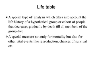
Life Table Survival Variable: Progression-Free Survival
ni
wi
di
No. of pts (13) began the
study, so n1 is 13
Interval
No.
No.
No.
No. of
Start entering withdrawn exposed terminal
2 patients are
Time
Interval
du.referredto risk
events
to as
Interval
withdrawals (w1).
qi = di/[ni- pi = 1–qi si = pipi–1pi(wi/2)]
2…p1
Propn
Propn
terminating surviving
Cumul Propn
Surv at End
0.0
13.0
2.0
12.0
1.0
1 patient's disease
0.0833 progressed, referred
0.9167
0.9167
to as a terminal
event (d1)
3.0
10.0
4.0
8.0
1.0
0.1250
0.8750
0.8021
6.0
5.0
4.0
3.0
0.0
0.0000
1.0000
0.8021
9.0
1.0
1.0
0.5
0.0
0.0000
1.0000
0.8021
Source: Noda K, Nishiwaki Y, Kawahara M, Negoro S, Sugiura T, Yokoyama A, et al: Irinotecan plus cisplatin
compared with etoposide plus cisplatin for extensive small-cell lung cancer. N Engl J Med 2002; 346: 85–

35. Assumption:
• The actuarial method assumes that patients withdraw
randomly throughout the interval; therefore, on the
average, they withdraw halfway through the time
represented by the interval.
• In a sense, this method gives patients who withdraw credit
for being in the study for half of the period.

36. Life table for sample of 13 patient treated with etoposide with cisplatin
Life Table Survival Variable: Progression-Free Survival
ni
wi
Interval
No.
No.
Start entering withdrawn
Time
Interval
du.
Interval
One-half of the number of patients
di
qi = di/[niwithdrawing is subtracted from the pi = 1–qi
(wi/2)]
number beginning the interval, so the
EXPOSED TO RISK during the
period, 13 – No. of2), or 12 in first
(½
No.
Propn
Propn
interval. terminal terminating surviving
exposed
to risk
si = pipi–1pi2…p1
Cumul Propn
Surv at End
events
0.0
13.0
2.0
12.0
1.0
0.0833
0.9167
0.9167
3.0
10.0
4.0
8.0
1.0
0.1250
0.8750
0.8021
6.0
5.0
4.0
3.0
0.0
0.0000
1.0000
0.8021
9.0
1.0
1.0
0.5
0.0
0.0000
1.0000
0.8021
Source: Noda K, Nishiwaki Y, Kawahara M, Negoro S, Sugiura T, Yokoyama A, et al: Irinotecan plus cisplatin
compared with etoposide plus cisplatin for extensive small-cell lung cancer. N Engl J Med 2002; 346: 85–

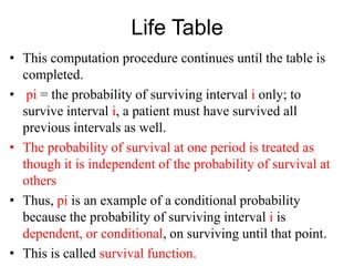
37. Life table for sample of 13 patient treated with etoposide with cisplatin
Life Table Survival Variable: Progression-Free Survival
ni
wi
Interval
No.
No.
Start entering withdrawn
Time
Interval
du.
Interval
di
No.
exposed
to risk
qi = di/[ni- pi = 1–qi si = pipi–1pi(wi/2)]
2…p1
The of
No. proportion terminating (q1
Propn
Propn
= d1/[n1-(w1/2]) is 1/12 =
terminal terminating surviving
0.0833.
events
Cumul Propn
Surv at End
0.0
13.0
2.0
12.0
1.0
0.0833
0.9167
0.9167
3.0
10.0
4.0
8.0
1.0
0.1250
0.8750
0.8021
6.0
5.0
4.0
3.0
0.0
0.0000
1.0000
0.8021
9.0
1.0
1.0
0.5
0.0
0.0000
1.0000
0.8021
Source: Noda K, Nishiwaki Y, Kawahara M, Negoro S, Sugiura T, Yokoyama A, et al: Irinotecan plus cisplatin
compared with etoposide plus cisplatin for extensive small-cell lung cancer. N Engl J Med 2002; 346: 85–

38. Life table for sample of 13 patient treated with etoposide with cisplatin
Life Table Survival Variable: Progression-Free Survival
ni
wi
Interval
No.
No.
Start entering withdrawn
Time
Interval
du.
Interval
di
No.
exposed
to risk
qi = di/[ni- pi = 1–qi si = pipi–1pi(wi/2)]
2…p1
No. of
Propn
Propn
Cumul Propn
terminal proportion surviving (p1 = 1-q1) is 1End
Surv at –
The terminating surviving
events
0.0833 = 0.9167
0.0
13.0
2.0
12.0
1.0
0.0833
0.9167
3.0
10.0
4.0
8.0
1.0
0.1250
0.8750 we are still in
0.8021
because
6.0
5.0
4.0
3.0
0.0
0.0000
9.0
1.0
1.0
0.5
0.0
0.0000
0.9167
the first period, the
cumulative survival is
1.0000
0.8021
0.9167
1.0000
0.8021
Source: Noda K, Nishiwaki Y, Kawahara M, Negoro S, Sugiura T, Yokoyama A, et al: Irinotecan plus cisplatin
compared with etoposide plus cisplatin for extensive small-cell lung cancer. N Engl J Med 2002; 346: 85–

39. Life table for sample of 13 patient treated with etoposide with cisplatin
Life Table Survival Variable: Progression-Free Survival
ni
wi
di
Interval
No.
No.
No.
No. of
the
Start At entering withdrawn exposed terminal
Time beginning of
Interval
du.
to risk
events
the second
four
Interval patients
withdraw w2 = 4
interval, only
0.0 10 patients
13.0
2.0
12.0
1.0
remain.n2=10
3.0
10.0
4.0
8.0
1.0
6.0
5.0
4.0
3.0
0.0
9.0
1.0
1.0
0.5
0.0
qi = di/[ni- pi = 1–qi si = pipi–1pi(wi/2)]
2…p1
Propn
Propn
terminating surviving
0.0833
0.9167
one's
0.1250
0.8750
disease
progressed,
so d2 = 1
Cumul Propn
Surv at End
0.9167
0.8021
0.0000
1.0000
0.8021
0.0000
1.0000
0.8021
Source: Noda K, Nishiwaki Y, Kawahara M, Negoro S, Sugiura T, Yokoyama A, et al: Irinotecan plus cisplatin
compared with etoposide plus cisplatin for extensive small-cell lung cancer. N Engl J Med 2002; 346: 85–

40. Life table for sample of 13 patient treated with etoposide with cisplatin
Life Table Survival Variable: Progression-Free Survival
ni
wi
di
Interval
No.
No.
No.
No. of
Start entering withdrawn exposed terminal
Time
Interval
du.
to risk
events
Interval
the proportion terminating (q2
nd
0.0
13.0 = d2/[n2-(w2/2]) during 2
2.0
12.0
1.0
interval is 1/[10 – (4/2)] =
1/8, or 0.1250.
qi = di/[ni- pi = 1–qi si = pipi–1pi(wi/2)]
2…p1
Propn
Propn proportion
the Cumul Propn
terminating surviving no
with Surv at End
progression is
1 – 0.1250, or
0.8750 0.9167
0.0833
0.9167
3.0
10.0
4.0
8.0
1.0
0.1250
0.8750
0.8021
6.0
5.0
4.0
3.0
0.0
0.0000
1.0000
0.8021
9.0
1.0
1.0
0.5
0.0
0.0000
1.0000
0.8021
Source: Noda K, Nishiwaki Y, Kawahara M, Negoro S, Sugiura T, Yokoyama A, et al: Irinotecan plus cisplatin
compared with etoposide plus cisplatin for extensive small-cell lung cancer. N Engl J Med 2002; 346: 85–

41. Life table for sample of 13 patient treated with etoposide with cisplatin
Life Table Survival Variable: Progression-Free Survival
ni
wi
Interval
No.
No.
Start entering withdrawn
Time
Interval
du.
Interval
0.0
3.0
13.0
10.0
2.0
di
No.
exposed
to risk
No. of
terminal
events
qi = di/[ni- pi = 1–qi si = pipi–1pi(wi/2)]
2…p1
Propn
Propn
terminating surviving
the
12.0 cumulative proportion of surv
1.0
0.0833
0.9167
4.0
8.0
6.0 from probability theory:
5.0
4.0
Rule
3.0
=p1*p2= 0.0.9167 × 0.8750=
0.8021
Cumul Propn
Surv at End
0.9167
1.0
0.1250
0.8750
0.8021
0.0
0.0000
1.0000
0.8021
0.0
0.0000
1.0000
0.8021
P(A&B)=P(A)*P(B) if A and B independent
9.0
1.0
1.0
0.5
Source: Noda K, Nishiwaki Y, Kawahara M, Negoro S, Sugiura T, Yokoyama A, et al: Irinotecan plus cisplatin
compared with etoposide plus cisplatin for extensive small-cell lung cancer. N Engl J Med 2002; 346: 85–9

42. Life table
• Like Cancer treatment, life table of survivorship after any
treatment as treatment of cancer by irradiation or drugs or
after operation, such as of cancer cervix or breast can be
prepared & made use in probabilities of survival at
beginning or at any point of time.
• More recently, survival can be enquired after– Heart operation like bypass, angioplasty, ballooning,
stenting, heart transplantation.
– Kidney, lung, liver & other organ transplantation.

43. Life Table
• This computation procedure continues until the table is
completed.
• pi = the probability of surviving interval i only; to
survive interval i, a patient must have survived all
previous intervals as well.
• The probability of survival at one period is treated as
though it is independent of the probability of survival at
others
• Thus, pi is an example of a conditional probability
because the probability of surviving interval i is
dependent, or conditional, on surviving until that point.
• This is called survival function.

44. Limitation
• The assumption that all withdrawals during a given
interval occur, on average, at the midpoint of the
interval.
• This assumption is of less consequence when short
time intervals are analyzed; however, considerable
bias can occur :
• if the intervals are large,
• if many withdrawals occur, &
• if withdrawals do not occur midway in the
interval.
• The Kaplan–Meier method overcomes this problem.

45. Kaplan Meier product limit method

46. Kaplan-Meier Product limit method
• Similar to actuarial analysis except time since entry in
the study is not divided into intervals for analysis.
• Survival is estimated each time a patient has an event.
• Withdrawals are ignored
• It gives exact survival times in comparison to
actuarial because it does not group survival time into
intervals
46

47. Introduction to Kaplan-Meier
• Non-parametric estimate of the survival function.
• Commonly used to describe survivorship of study
population/s.
• Commonly used to compare two study populations.
• Intuitive graphical presentation.
47

48. Survival Data (right-censored)
Subject A
Subject B
Subject C
Subject D
Subject E
X 1. subject E dies at 4
months
0
Beginning of study
12
 Time in months 
End of study

49. Corresponding Kaplan-Meier Curve
100%
Probability of
surviving to 4
months is 100% =
5/5
Fraction
surviving this
death = 4/5
Subject E dies at 4
months
4
 Time in months 

50. Survival Data
Subject A
Subject B
2. subject A
drops out after
6 months
Subject C
3. subject C dies
X at 7 months
Subject D
Subject E
X 1. subject E dies at 4
months
Beginning of study
 Time in months 
End of study

51. Corresponding Kaplan-Meier Curve
100%
Fraction
surviving this
death = 2/3
subject C dies at
7 months
4
7
 Time in months 

52. Survival Data
Subject A
2. subject A
drops out after
6 months
Subject B
3. subject C dies
X at 7 months
Subject C
Subject D
Subject E
4. Subjects B
and D survive
for the whole
year-long
study period
X 1. subject E dies at 4
months
Beginning of study
 Time in months 
End of study

53. Corresponding Kaplan-Meier Curve
Rule from probability theory:
100%
P(A&B)=P(A)*P(B) if A and B independent
In kaplan meier : intervals are defined by failures(2 intervals leading to failures here).
P(surviving intervals 1 and 2)=P(surviving interval 1)*P(surviving interval 2)
Product limit estimate of survival =
P(surviving interval 1/at-risk up to failure 1) *
P(surviving interval 2/at-risk up to failure 2)
= 4/5 * 2/3= .5333
The probability of surviving in the entire year, taking into account
censoring
= (4/5) (2/3) = 53%
0
 Time in months 
12

54. Example :kaplan–Meier survival curve in detail for
patients on etoposide plus cisplatin
Event
Time
(T)
Number at
Risk
ni
Number of
Events
di
Mortality
qi = di/ni
Survival
pi = 1 - qi
Cumulative Survival
S = pip(i-1)…p2p1
1.0
13
1
0.076
0.9231
0.9231
2.4
12
2.8
11
3.1
10
3.7
9
4.4
8
4.6
7
4.7
6
6.5
5
7.1
4
8.0
3
8.1
2
12.0
1
• In this method first step is to list the times when a death or drop
out occurs, as in the column “Event Time”.
1
0.1250
0.8750
0.8077
• One patient's disease progressed at 1 month and another at 4.4
months, and they are listed under the column “Number of Events.”
• Then, each time an event or outcome occurs, the mortality,
survival, and cumulative survival are calculated in the same
manner as with the life table method.

55. Contd…
• If the table is published in an article, it is often
formatted in an abbreviated form, such as in Table 5.
Kaplan–Meier survival curve in abbreviated form for patients on etoposide plus
cisplatin
Event Time
(T)
Number at
Risk
ni
Number of
Events
di
Mortality
qi = di/ni
Survival
pi = 1 - qi
Cumulative Survival
S = pip(i-1)…p2p1
1.0
13
1
0.076
0.9231
0.9231
4.4
8
1
0.1250
0.8750
0.8077
..
..
..
12.0

56. 2.0
4.0
6.0
8.0
10.0
12.0
Kaplan meir survival curve for patients on etoposide & cisplatin
(Source: Source: Noda K, Nishiwaki Y, Kawahara M, Negoro S, Sugiura T, Yokoyama A, et al: Irinotecan
plus cisplatin compared with etoposide plus cisplatin for extensive small-cell lung cancer. N Engl J Med
2002; 346: 85–91.)

57. Limitations of Kaplan-Meier
• Requires nominal predictors only
• Doesn‟t control for covariates
Cox progressive hazard model solves these problems
57

58. Kaplan meir survival curve with 95 % confidence limits for
patients on irinotecan & cisplatin
(Source: Source: Noda K, Nishiwaki Y, Kawahara M, Negoro S, Sugiura T, Yokoyama A, et al:
Irinotecan plus cisplatin compared with etoposide plus cisplatin for extensive small-cell lung
cancer. N Engl J Med 2002; 346: 85–91.)

59. Comparison between 2 survival
curve
• Don’t make judgments simply on
the basis of the amount of
separation between two lines

60. Comparison between 2 survival
curve
• For comparison if no censored observations
occur, the Wilcoxon rank sum test introduced,
is appropriate for comparing the ranks of
survival time.
• If some observations are censored, methods
may be used to compare survival curves.
– the Logrank statistic
– the Mantel–Haenszel chi-square statistic.

61. Logrank test
• The log rank statistic is one of the most
commonly used methods to learn if two curves
are significantly different.
• This method also known as Mantel-logrank
statistics or Cox-Mantel-logrank statistics
• The logrank test compares the number of
observed deaths in each group with the number of
deaths that would be expected based on the
number of deaths in the combined groups that is,
if group membership did not matter.

62. Hazard ratio
• The logrank statistic calculates the hazard ratio
• It is estimated by O1st group/E1st group
divided by O2nd group/E2group
• The hazard ratio is interpreted in a similar
manner as the odds ratio
• Using the hazard ratio assumes that the hazard
or risk of death is the same throughout the time
of the study.

63. Mantel– Haenszel chi test
• Another method for comparing survival distributions is
an estimate of the odds ratio developed by Mantel and
Haenszel that follows (approximately) a chi-square
distribution with 1 degree of freedom.
• The Mantel– Haenszel test combines a series of 2 2
tables formed at different survival times into an overall
test of significance of the survival curves.
• The Mantel–Haenszel statistic is very useful because it
can be used to compare any distributions, not simply
survival curves

64. Cox progressive hazard model

65. Why is called cox proportional
hazard model
• Cox =scientist‟s name(Sir David Roxbee Cox)
– British statistician
– In 1972 developed it.
• Uses hazard function
• covariates have a multiplicative or a proportional ,
effect on the probability of event

66. What does cox model do>
• It examines two pieces of information:
– The amount of time since the event first happened
to a person
– The person‟s observations on the independent
variables.

67. Cox progressive hazard model
• Used to assess the simultaneous effect of
several variables on length of survival.
• It allows the covariates(independent variables)
in the regression equation to vary with time.
• Both numerical and nominal independent
variables may be used in this model.

68. COX regression coefficient
• Determines relative risk or odd‟s ratio
associated with each independent variable and
outcome variable, adjusted for the effect of all
other variables .

69. Hazard function
• Opposite to survival function
• Hazard function is the derivative of the survival
function over time h(t)=dS(t)/dt
• instantaneous risk of event at time t (conditional
failure rate)
• It is the probability that a person will die in the next
interval of time, given that he survived until the
beginning of the interval.

70. Hazard function
• Hazard function given by
h(t,x1,x2…x5)=ƛ0 (t)eb1x1+b2x2+….b5x5
• ƛ0 is the baseline hazard at time t i.e. ƛ0(t)
• For any individual subject the hazard at time t is hi(t).
• hi(t) is linked to the baseline hazard h0(t) by
loge {hi(t)} = loge{ƛ0(t)} + β1X1 + β2X2 +……..+ βpXp
• where X1, X2 and Xp are variables associated with the
subject

71. Proportional hazards:
Hazard ratio
Hazard for person i (eg a smoker)
hi (t ) 0 (t )e 1xi1 ...  k xik
 ( x  x ) ... 1 ( xik  x jk )
HRi , j 

 e 1 i1 j 1
h j (t ) 0 (t )e 1x j1 ...  k x jk
Hazard for person j (eg
a non-smoker)
Hazard functions should be strictly parallel!
Produces covariate-adjusted hazard ratios!
71

72. The model: binary predictor

HRlung cancer/ smoking
(1)  
hi (t ) 0 (t )e smoking age

(10 )


 e smoking
h j (t ) 0 (t )e  smoking ( 0)  age ( 60)
HRlung cancer/ smoking  e
( 60 )
 smoking
This is the hazard ratio for smoking adjusted for age.
72

73. Table 2. Death rates for screenwriters who have won an
academy award.* Values are percentages (95% confidence
intervals) and are adjusted for the factor indicated
Basic analysis
Adjusted analysis
Demographic:
Year of birth
Relative increase
in death rate for
winners
37 (10 to 70)
HR=1.37; interpretation:
37% higher incidence of
death for winners compared
with nominees
32 (6 to 64)
Sex
36 (10 to 69)
Documented education
39 (12 to 73)
All three factors
33 (7 to 65)
Professional:
Film genre
Total films
Total four star films
Total nominations
Age at first film
HR=1.35; interpretation:
35% higher incidence of
death for winners compared
with nominees even after
adjusting for potential
confounders
37 (10 to 70)
39 (12 to 73)
40 (13 to 75)
43 (14 to 79)
36 (9 to 68)
Age at first nomination
32 (6 to 64)
All six factors
40 (11 to 76)
All nine factors
35 (7 to 70)

74. Importance
• Provides the only valid method of predicting a
time dependent outcome , and many health
related outcomes related to time.
• Can be interpreted in relative risk or odds ratio
• Gives survival curves with control of
confounding variables.
• Can be used with multiple events for a subject.

75. Take Home Message
• survival analysis deals with situations where
the outcome is dichotomous and is a function
of time
• In survival data is transformed into censored
and uncensored data
• all those who achieve the outcome of interest
are uncensored” data
• those who do not achieve the outcome are
“censored” data

76. Take Home Message
• The actuarial method adopts fixed class intervals
which are most often year following the end of
treatment given.
• The Kaplan-Meier method uses the next
death, whenever it occurs, to define the end of the last
class interval and the start of the new class interval.
• Log-Rank test used to compare 2 survival curves but
does not control for confounding.
• Mantel henzel test can compare any curve not only
survial curves
• For control for confounding use another test called as
„Cox Proportional Hazards Regression.’

77. Thank you