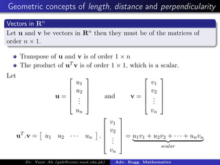
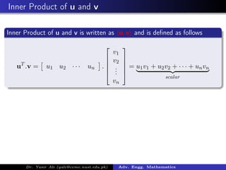
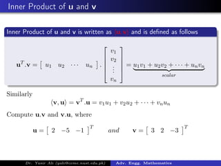
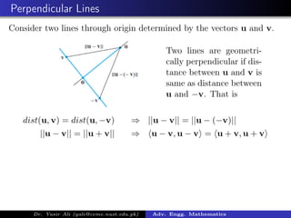
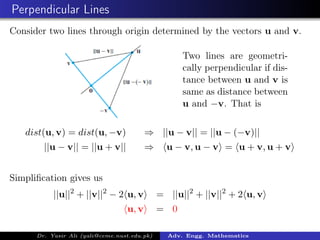
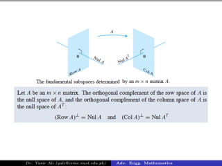
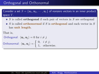
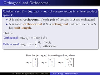
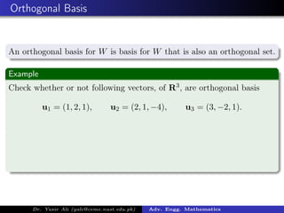
This document discusses orthogonal subspaces and inner products in advanced engineering mathematics. It defines the inner product of two vectors u and v in Rn as the transpose of u dotted with v, which results in a scalar. Two vectors are orthogonal if their inner product is 0. An orthogonal basis for a subspace W is a basis for W that is also an orthogonal set. The document also discusses orthogonal complements, projections, and inner products on function spaces.
- Quiz 4 will be tomorrow covering sections 3.3, 5.1, and 5.2 of the textbook. It will include 3 problems on Cramer's rule, finding eigenvectors given eigenvalues, and finding characteristic polynomials/eigenvalues of 2x2 and 3x3 matrices. Students must show all work.
- Chapter 6 objectives include extending geometric concepts like length, distance, and perpendicularity to Rn. These concepts are useful for least squares fitting of experimental data to a system of equations.
- The inner product of two vectors u and v in Rn is defined as their dot product, which is the sum of the component-wise products of corresponding elements in u and v.
The document discusses closures of relations, including reflexive closure and symmetric closure. It provides definitions and theorems related to closures. It also uses an example to illustrate finding the reflexive closure and symmetric closure of a relation. Additionally, it covers topics like paths in directed graphs, shortest paths, and transitive closure. It includes an example of calculating the transitive closure of a relation by finding its zero-one matrix.
Application of Matrices in real life | Matrices application | The MatricesSahilJhajharia
Matrices can be used to transform vectors by changing their magnitude and direction. Matrices are useful for applications like rotating vectors, solving systems of linear equations, and encoding/decoding messages for cryptography. As an example, a message can be encoded using a matrix, transmitted as encoded values, and then decoded by the receiver using the inverse matrix. Eigenvectors are vectors that only change in magnitude and not direction when multiplied by a matrix. They can be used to model real-world systems changing over time, like populations of humans and zombies.
The document discusses inner product spaces and orthonormal bases. It defines an inner product space as a vector space with an inner product defined on it. An orthonormal basis is introduced as a set of orthogonal unit vectors that form a basis. The Gram-Schmidt process is presented as a method for transforming a basis into an orthonormal basis. Properties of inner products, such as the Cauchy-Schwarz inequality and orthogonal projections, are covered.
(1) The document discusses inner product spaces and related linear algebra concepts such as orthogonal vectors and bases, Gram-Schmidt process, orthogonal complements, and orthogonal projections.
(2) Key topics covered include defining inner products and their properties, finding orthogonal vectors and constructing orthogonal bases, using Gram-Schmidt process to orthogonalize a set of vectors, defining and finding orthogonal complements of subspaces, and computing orthogonal projections of vectors.
(3) Examples are provided to demonstrate computing orthogonal bases, orthogonal complements, and orthogonal projections in inner product spaces.
The document discusses vector calculus concepts including:
1) Coordinate systems used in vector calculus problems including rectangular, cylindrical, and spherical coordinates.
2) How to write vectors and their components in each coordinate system.
3) Relationships between vectors in different coordinate systems using transformation matrices.
4) Concepts of gradient, divergence, and curl and their definitions and representations in different coordinate systems.
5) Theorems relating integrals, including the divergence theorem and Stokes' theorem.
The document provides an overview of vector spaces and related linear algebra concepts. It defines vector spaces, subspaces, basis, dimension, and rank. Key points include:
- A vector space is a set that is closed under vector addition and scalar multiplication. It must satisfy certain axioms.
- A subspace is a subset of a vector space that is also a vector space.
- A basis is a minimal set of linearly independent vectors that span the entire vector space. The dimension of a vector space is the number of vectors in its basis.
- The rank of a matrix is the number of linearly independent rows in its row-reduced echelon form. It provides a measure of the matrix's linear
The document discusses various topics in graph theory including definitions, types, and applications of graphs. It covers definitions of graphs, edges, degrees, paths and connectivity. Graph representations like adjacency matrix and lists are presented. Different types of graphs are defined including simple, multigraphs, pseudographs, directed graphs. Special graph structures like trees, cycles, wheels and n-cubes are discussed along with theorems on handshaking and degrees in graphs. Bipartite graphs and graph isomorphism are also covered.
Here are the key steps to find the eigenvalues of the given matrix:
1) Write the characteristic equation: det(A - λI) = 0
2) Expand the determinant: (1-λ)(-2-λ) - 4 = 0
3) Simplify and factor: λ(λ + 1)(λ + 2) = 0
4) Find the roots: λ1 = 0, λ2 = -1, λ3 = -2
Therefore, the eigenvalues of the given matrix are -1 and -2.
This experiment aims to determine the Hall coefficient of a semiconductor sample using the Hall effect. A rectangular semiconductor sample is placed in a perpendicular magnetic and electric field. Charges in the sample experience a Lorentz force, causing a potential difference called the Hall voltage to develop across the sample. Hall voltage measurements are taken at varying currents through the sample. The Hall coefficient is then calculated from the slope of the Hall voltage-current graph and used to characterize the semiconductor by determining the type and concentration of charge carriers in the sample. Precautions are taken to accurately measure and control the magnetic field and avoid sample heating.
This document discusses linear transformations and their properties. It defines a linear transformation as a function between vector spaces that preserves vector addition and scalar multiplication. The kernel of a linear transformation is the set of vectors mapped to the zero vector, and is a subspace of the domain. The range is the set of images of all vectors under the transformation. Matrices can represent linear transformations, with the matrix equation representing the transformation of vectors. Examples are provided to illustrate key concepts such as kernels, ranges, and matrix representations of linear transformations.
This document discusses complex numbers including:
1. Defining complex numbers and their algebraic properties such as addition, subtraction, multiplication and division.
2. Geometrically representing complex numbers in Cartesian and polar forms.
3. Key concepts such as the absolute value, distance between complex numbers, and the interpretation of multiplication in polar form.
4. De Moivre's theorem and its expansion along with examples of evaluating complex numbers and finding roots of complex numbers using this theorem.
5. Exponential and logarithmic forms of representing complex numbers.
This document discusses the Gamma and Beta functions. It defines them using improper definite integrals and notes they are special transcendental functions. The Gamma function was introduced by Euler and both functions have applications in areas like number theory and physics. The document provides properties of each function and examples of evaluating integrals using their definitions and relations.
This document discusses using matrices for cryptography. It explains that encryption involves transforming data into an unreadable form using a key, while decryption reverses the process. For matrix cryptography, a message is converted to numbers and broken into vectors, which are then encoded by multiplying with an encoding matrix. The encoded message is transmitted and decoded by the receiver by multiplying the vectors with the inverse decoding matrix. When decoded, the original message is revealed.
Transformation matrices can be used to describe that at what angle the servos need to be to reach the desired position in space or may be an underwater autonomous vehicle needs to reach or align itself with several different obstacles inside the water.
This document provides an introduction and overview of a discrete mathematics course. It explains that discrete mathematics lays the mathematical foundations for many computer science topics. It lists common topics covered in the course like logic, sets, functions, counting, recursion, graphs and trees. It emphasizes that discrete mathematics deals with discrete, distinct objects like those used in computing. Mastering this subject involves actively practicing the concepts rather than just hearing or reading about them.
LU decomposition is a method to solve systems of linear equations by decomposing the coefficient matrix A into the product of a lower triangular matrix L and an upper triangular matrix U. It involves (1) decomposing A into L and U, (2) solving LZ = C for Z, and (3) solving UX = Z for X to find the solution vector X. The document provides an example using LU decomposition to solve a system of 3 linear equations.
Engineering mathematics applies mathematical theory to complex real-world engineering problems through practical engineering, scientific computing, and combining traditional boundaries. Matrices were first formulated in 1850 and organize numbers and variables in a rectangular structure. They are widely used across many fields including chemistry to balance chemical equations represented as matrices, electrical circuits using Kirchhoff's laws, computer graphics for transformations, graph theory, cryptography through encoding/decoding matrices, seismic surveys, robotics for programming movements, analyzing forces on bridges, and recording data and reports.
MATLAB is a programming language for technical computing and data analysis. It allows users to perform arithmetic operations, use mathematical functions, manipulate data, create plots and graphs, write programs using conditional statements and loops. The document provides an overview of MATLAB's interface and important terms, and demonstrates how to perform common tasks like creating arrays and matrices, plotting data, writing for and while loops, and defining functions. MATLAB is relevant for tasks in many engineering fields like signal processing, optimization, finite element analysis, and statistical analysis.
This document provides notes on vector spaces, which are fundamental objects in linear algebra. It begins with examples of vector spaces such as R2, R3, C2, C3 and defines vector spaces more generally as sets that are closed under vector addition and scalar multiplication and satisfy other properties like the existence of additive identities. It then provides several examples of vector spaces including the set of all n-tuples over a field, the set of all m×n matrices, the set of differentiable functions on an interval, and the set of polynomials with coefficients in a field.
The document discusses different types of topological spaces, including Hausdorff and non-Hausdorff spaces. It defines separation axioms like T0, T1, T2, etc. and explains that metric spaces and the real number line are Hausdorff. Non-Hausdorff spaces are exemplified using an equivalence relation on the space [0,1]∪[2,3]. Regular, normal and compact Hausdorff spaces are also discussed.
1) Stokes' theorem relates a surface integral over a surface S to a line integral around the boundary curve of S. It states that the line integral of a vector field F around a closed curve C that forms the boundary of a surface S is equal to the surface integral of the curl of F over the surface S.
2) In Example 1, Stokes' theorem is used to evaluate a line integral around an elliptical curve C by calculating the corresponding surface integral over the elliptical region S bounded by C.
3) In Example 2, Stokes' theorem is again used, this time to evaluate a line integral around a circular curve C by calculating the surface integral over the part of a sphere bounded by C.
The following presentation consists of information about the application of matrices. The ppt particularly focuses on the its use in cryptography i.e. encoding and decoding of messages.
In this presentation we will learn Del operator, Gradient of scalar function , Directional Derivative, Divergence of vector function, Curl of a vector function and after that solved some example related to above.
Gradient in math
Directional derivative in math
Divergence in math
Curl in math
Gradient , Directional Derivative , Divergence , Curl in mathematics
Gradient , Directional Derivative , Divergence , Curl in math
Gradient , Directional Derivative , Divergence , Curl
1. The orthogonal decomposition theorem states that any vector y in Rn can be written uniquely as the sum of a vector ŷ in a subspace W and a vector z orthogonal to W.
2. The vector ŷ is called the orthogonal projection of y onto W. It is the closest vector to y that lies in W.
3. The best approximation theorem states that the orthogonal projection ŷ provides the best or closest approximation of y using only vectors that lie in the subspace W. The distance from y to ŷ is less than the distance from y to any other vector in
This document defines vectors and scalar quantities, and describes their key properties and relationships. It begins by defining physical quantities that can be measured, and distinguishes between scalar and vector quantities. Scalars have only magnitude, while vectors have both magnitude and direction. The document then provides a more rigorous definition of vectors as quantities that remain invariant under coordinate system rotations or translations. It describes how to represent and transform vectors between different coordinate systems. Vector addition, subtraction, and multiplication operations like the scalar and vector products are defined. Derivatives of vectors are also discussed. Examples of velocity and acceleration vectors in uniform circular motion are provided.
This document discusses the Gram-Schmidt orthogonalization (GSO) process. It provides three examples: 1) defining orthogonal vectors and orthogonal matrices, 2) finding the coefficient and projection of a vector onto another vector, and 3) using GSO to transform a basis into an orthonormal basis in R3 space.
In this paper, natural inner product structure for the space of fuzzy n−tuples is introduced. Also we have
introduced the ortho vector, stochastic fuzzy vectors, ortho- stochastic fuzzy vectors, ortho-stochastic fuzzy
matrices and the concept of orthogonal complement of fuzzy vector subspace of a fuzzy vector space.
Linear Transformation Vector Matrices and SpacesSohaib H. Khan
The document discusses linear transformations between vector spaces. It defines a linear transformation as a mapping between vector spaces that satisfies two conditions: 1) it is additive and 2) it is homogeneous. It also defines the kernel as the set of vectors that map to the zero vector, and the image as the set of vectors in the target space that are the image of vectors in the domain space. The document is about linear transformations presented by Dr. Yasir Ali for an advanced engineering mathematics course.
The document verifies properties of the scalar and vector product in R3 using general vector expressions.
It first proves six properties of the dot product: 1) distributivity over vector addition, 2) commutativity, 3) the formula for vector length, 4) distributivity of scalar multiplication, 5) the dot product between a non-zero vector and the zero vector is zero, and 6) if the dot product of a vector with itself is zero, then the vector is the zero vector.
It then proves one property of the cross product: the length of the cross product of two vectors is equal to the product of the lengths of the vectors multiplied by the sine of the angle between them.
2. Linear Algebra for Machine Learning: Basis and DimensionCeni Babaoglu, PhD
The seminar series will focus on the mathematical background needed for machine learning. The first set of the seminars will be on "Linear Algebra for Machine Learning". Here are the slides of the second part which is discussing basis and dimension.
Here is the link of the first part which was discussing linear systems: https://www.slideshare.net/CeniBabaogluPhDinMat/linear-algebra-for-machine-learning-linear-systems/1
This document provides an introduction and overview of vectors. It begins by defining a vector as an object with both magnitude and direction. It then discusses various vector concepts such as addition, scalar multiplication, standard basis vectors, and unit vectors. Examples are provided to demonstrate vector operations and representations using coordinates. The document aims to introduce foundational vector concepts.
In this paper we introduce the concept of the spherical interval-valued fuzzy bi-ideal of gamma near-ring R and its some results. The union and intersection of the spherical interval-valued fuzzy bi-ideal of gamma near-ring R is also a spherical interval-valued fuzzy bi-ideal of gamma near-ring R . Further we discuss about the relationship between bi-ideal and spherical interval-valued fuzzy bi-ideal of gamma near-ring R.
This document summarizes a presentation on developing a natural finite element for axisymmetric problems. It introduces an axisymmetric model problem, defines appropriate axisymmetric Sobolev spaces, and presents a discrete formulation using a P1 finite element on triangles. Numerical results on a test problem show the method achieves the same convergence rates as classical approaches but with significantly smaller errors. The analysis draws on previous work to prove first-order approximation properties under certain mesh assumptions.
Chapter 12
Section 12.1: Three-Dimensional Coordinate Systems
We locate a point on a number line as one coordinate, in the plane as an ordered pair, and in
space as an ordered triple. So we call number line as one dimensional, plane as two
dimensional, and space as three dimensional co – ordinate system.
In three dimensional, there is origin (0, 0, 0) and there are three axes – x -, y - , and z – axis. X –
and y – axes are horizontal and z – axis is vertical. These three axes divide the space into eight
equal parts, called the octants. In addition, these three axes divide the space into three
coordinate planes.
– The xy-plane contains the x- and y-axes. The equation is z = 0.
– The yz-plane contains the y- and z-axes. The equation is x = 0.
– The xz-plane contains the x- and z-axes. The equation is y = 0.
If P is any point in space, let:
– a be the (directed) distance from the yz-plane to P.
– b be the distance from the xz-plane to P.
– c be the distance from the xy-plane to P.
Then the point P by the ordered triple of real numbers (a, b, c), where a, b, and c are the
coordinates of P.
– a is the x-coordinate.
– b is the y-coordinate.
– c is the z-coordinate.
– Thus, to locate a point (a, b, c) in space, start from the origin (0, 0, 0) and move a
units along the x-axis. Then, move b units parallel to the y-axis. Finally, move c
units parallel to the z-axis.
The three dimensional Cartesian co – ordinate system follows the right hand rule.
Examples:
Plot the points (2,3,4), (2, -3, 4), (-2, -3, 4), (2, -3, -4), and (-2, -3, -4).
The Cartesian product x x = {(x, y, z) | x, y, z in } is the set of all ordered triples of
real numbers and is denoted by 3 .
Note:
1. In 2 – dimension, an equation in x and y represents a curve in the plane 2 . In 3 –
dimension, an equation in x, y, and z represents a surface in space 3 .
2. When we see an equation, we must understand from the context that it is a curve in the
plane or a surface in space. For example, y = 5 is a line in 2 �but it is a plane in 3 �
������
3. in space, if k, l, & m are constants, then
– x = k represents a plane parallel to the yz-plane ( a vertical plane).
– y = k is a plane parallel to the xz-plane ( a vertical plane).
– z = k is a plane parallel to the xy-plane ( a horizontal plane).
– x = k & y = l is a line.
– x = k & z = m is a line.
– y = l & z = m is a line.
– x = k, y = l and z = m is a point.
Examples: Describe and sketch y = x in 3
Example:
Solve:
Which of the points P(6, 2, 3), Q(-5, -1, 4), and R(0, 3, 8) is closest to the xz – plane? Which point
lies in the yz – plane?
Distance between two points in space:
We simply extend the formula from 2 to . 3 . The distance |p1 p2 | between the points
P1(x1,y1, z1) and P2(x2, y2, z2) is: 2 2 21 2 2 1 ...
The document provides an overview of vector spaces and related concepts:
(1) Historically, ideas around vector spaces date back to the 17th century but received a more abstract treatment in 1888 by Giuseppe Peano. Key developments include Grassmann introducing vector spaces in 1844 and Peano providing a definition of vector spaces and linear maps.
(2) A vector space is a set that is closed under vector addition and scalar multiplication. It allows objects called vectors to be added and multiplied by numbers called scalars. Real numbers are often used as scalars but other fields can also be used.
(3) For a set to be a vector space, the basic operations of vector addition and scalar multiplication must satisfy
The document discusses orthogonal bases and the Gram-Schmidt process. It defines the Gram-Schmidt process as an algorithm for finding an orthogonal basis from a given basis by making each new vector orthogonal to the previous ones. It also discusses orthonormal bases, QR factorization, inner products, length and distance, and applying Gram-Schmidt to produce an orthogonal basis for the vector space of polynomials up to degree 2.
The document discusses similarity transformations and the Cauchy-Schwarz inequality. It states that if matrix A is similar to matrix B, then B is similar to A, and if A is similar to B and B is similar to C, then A is similar to C. It also proves that if A is similar to B, then the inverse of A is similar to the inverse of B. Additionally, it defines the inner product and norm of vectors, and proves the Cauchy-Schwarz inequality that the square of the inner product of two vectors is less than or equal to the product of their norms. It provides an example using the Cauchy-Schwarz inequality to prove an inequality involving positive real numbers.
The International Journal of Engineering & Science is aimed at providing a platform for researchers, engineers, scientists, or educators to publish their original research results, to exchange new ideas, to disseminate information in innovative designs, engineering experiences and technological skills. It is also the Journal's objective to promote engineering and technology education. All papers submitted to the Journal will be blind peer-reviewed. Only original articles will be published.
The document discusses linear independence and change of basis in vector spaces. It provides the following key points:
1) Two vectors u and v are linearly dependent if one is a multiple of the other, and independent otherwise.
2) Three vectors u, v, and w are linearly dependent if their coefficients in a linear combination equal 0, and independent otherwise.
3) A change of basis matrix P describes the transformation between two bases {e} and {f} of a vector space, where each vector in {f} is written as a linear combination of the vectors in {e}. The inverse of P transforms vectors back from {f} to {e}.
This article is interested to a detailed computation of the commutators of the Hopaf
algebra Uq(sl(n)). It can be treated as a second way to computation the brackets
of the Hopf algebra Uq(sl(n)) which could be introducing and understanding the
Uq(sl(n)) for the researchers.
1) The document discusses vector spaces and linear combinations. It defines a vector space as a set of objects called vectors that can be added together and multiplied by scalars, following certain properties like closure and the existence of additive inverses.
2) Examples of vector spaces include Rn (n-dimensional coordinate vectors), matrices, and sets of functions. A linear combination is an expression of a vector as a sum of other vectors multiplied by scalars.
3) The key characteristics of a vector space are that it is closed under vector addition and scalar multiplication, has an additive identity element (the zero vector), and vectors have additive inverses. Any set satisfying these properties forms a vector space.
The document discusses Lagrange interpolation, which involves constructing a polynomial that passes through a set of known data points. Specifically, it describes:
- The interpolation problem of predicting an unknown value (fI) at a point (xI) given known values (fi) at nodes (xi)
- How Lagrange interpolation polynomials are defined using basis polynomials (Ln,k) such that each basis polynomial is 1 at its node and 0 at other nodes
- An example of constructing a 3rd degree Lagrange interpolation polynomial to interpolate an unknown value f(3) using 4 known data points
The document discusses Lagrange interpolation and divided differences. It explains that the Lagrange interpolation polynomial can be written in terms of divided differences, where the coefficients are divided differences of the function values. Divided differences are defined recursively, and a pattern is identified to write them in terms of the function values at nodes. An example divided difference table is given for a set of data points.
Production Planning, Scheduling and ControlSohaib H. Khan
This document provides an overview of production scheduling and control. It discusses topics like introduction, aggregate production planning, demand forecasting, workforce planning, production routing, and production scheduling. The introduction defines production scheduling and control and its importance. Aggregate production planning involves medium-term planning to establish rough production levels. Demand forecasting predicts future requirements using qualitative, extrapolative, and causal methods. Workforce planning ensures the right workforce is available. Production routing determines the production path. Production scheduling sets timetables for manufacturing operations.
The document discusses the benefits of exercise for mental health. Regular physical activity can help reduce anxiety and depression and improve mood and cognitive function. Exercise causes chemical changes in the brain that may help protect against mental illness and improve symptoms for those who already suffer from conditions like anxiety and depression.
The document discusses the benefits of exercise for mental health. Regular physical activity can help reduce anxiety and depression and improve mood and cognitive functioning. Exercise causes chemical changes in the brain that may help boost feelings of calmness and well-being.
The document discusses the benefits of exercise for mental health. Regular physical activity can help reduce anxiety and depression and improve mood and cognitive functioning. Exercise causes chemical changes in the brain that may help boost feelings of calmness, happiness and focus.
The document discusses the benefits of exercise for mental health. Regular physical activity can help reduce anxiety and depression and improve mood and cognitive functioning. Exercise causes chemical changes in the brain that may help protect against developing mental illness and improve symptoms for those who already suffer from conditions like anxiety and depression.
The document discusses the benefits of exercise for mental health. Regular physical activity can help reduce anxiety and depression and improve mood and cognitive functioning. Exercise causes chemical changes in the brain that may help protect against mental illness and improve symptoms.
The document discusses the benefits of exercise for mental health. Regular physical activity can help reduce anxiety and depression and improve mood and cognitive functioning. Exercise causes chemical changes in the brain that may help protect against mental illness and improve symptoms for those who already suffer from conditions like anxiety and depression.
Main Java[All of the Base Concepts}.docxadhitya5119
This is part 1 of my Java Learning Journey. This Contains Custom methods, classes, constructors, packages, multithreading , try- catch block, finally block and more.
This slide is special for master students (MIBS & MIFB) in UUM. Also useful for readers who are interested in the topic of contemporary Islamic banking.
ISO/IEC 27001, ISO/IEC 42001, and GDPR: Best Practices for Implementation and...PECB
Denis is a dynamic and results-driven Chief Information Officer (CIO) with a distinguished career spanning information systems analysis and technical project management. With a proven track record of spearheading the design and delivery of cutting-edge Information Management solutions, he has consistently elevated business operations, streamlined reporting functions, and maximized process efficiency.
Certified as an ISO/IEC 27001: Information Security Management Systems (ISMS) Lead Implementer, Data Protection Officer, and Cyber Risks Analyst, Denis brings a heightened focus on data security, privacy, and cyber resilience to every endeavor.
His expertise extends across a diverse spectrum of reporting, database, and web development applications, underpinned by an exceptional grasp of data storage and virtualization technologies. His proficiency in application testing, database administration, and data cleansing ensures seamless execution of complex projects.
What sets Denis apart is his comprehensive understanding of Business and Systems Analysis technologies, honed through involvement in all phases of the Software Development Lifecycle (SDLC). From meticulous requirements gathering to precise analysis, innovative design, rigorous development, thorough testing, and successful implementation, he has consistently delivered exceptional results.
Throughout his career, he has taken on multifaceted roles, from leading technical project management teams to owning solutions that drive operational excellence. His conscientious and proactive approach is unwavering, whether he is working independently or collaboratively within a team. His ability to connect with colleagues on a personal level underscores his commitment to fostering a harmonious and productive workplace environment.
Date: May 29, 2024
Tags: Information Security, ISO/IEC 27001, ISO/IEC 42001, Artificial Intelligence, GDPR
-------------------------------------------------------------------------------
Find out more about ISO training and certification services
Training: ISO/IEC 27001 Information Security Management System - EN | PECB
ISO/IEC 42001 Artificial Intelligence Management System - EN | PECB
General Data Protection Regulation (GDPR) - Training Courses - EN | PECB
Webinars: https://pecb.com/webinars
Article: https://pecb.com/article
-------------------------------------------------------------------------------
For more information about PECB:
Website: https://pecb.com/
LinkedIn: https://www.linkedin.com/company/pecb/
Facebook: https://www.facebook.com/PECBInternational/
Slideshare: http://www.slideshare.net/PECBCERTIFICATION
it describes the bony anatomy including the femoral head , acetabulum, labrum . also discusses the capsule , ligaments . muscle that act on the hip joint and the range of motion are outlined. factors affecting hip joint stability and weight transmission through the joint are summarized.
How to Fix the Import Error in the Odoo 17Celine George
An import error occurs when a program fails to import a module or library, disrupting its execution. In languages like Python, this issue arises when the specified module cannot be found or accessed, hindering the program's functionality. Resolving import errors is crucial for maintaining smooth software operation and uninterrupted development processes.
How to Manage Your Lost Opportunities in Odoo 17 CRMCeline George
Odoo 17 CRM allows us to track why we lose sales opportunities with "Lost Reasons." This helps analyze our sales process and identify areas for improvement. Here's how to configure lost reasons in Odoo 17 CRM
A Strategic Approach: GenAI in EducationPeter Windle
Artificial Intelligence (AI) technologies such as Generative AI, Image Generators and Large Language Models have had a dramatic impact on teaching, learning and assessment over the past 18 months. The most immediate threat AI posed was to Academic Integrity with Higher Education Institutes (HEIs) focusing their efforts on combating the use of GenAI in assessment. Guidelines were developed for staff and students, policies put in place too. Innovative educators have forged paths in the use of Generative AI for teaching, learning and assessments leading to pockets of transformation springing up across HEIs, often with little or no top-down guidance, support or direction.
This Gasta posits a strategic approach to integrating AI into HEIs to prepare staff, students and the curriculum for an evolving world and workplace. We will highlight the advantages of working with these technologies beyond the realm of teaching, learning and assessment by considering prompt engineering skills, industry impact, curriculum changes, and the need for staff upskilling. In contrast, not engaging strategically with Generative AI poses risks, including falling behind peers, missed opportunities and failing to ensure our graduates remain employable. The rapid evolution of AI technologies necessitates a proactive and strategic approach if we are to remain relevant.
1. Adv. Engg. Mathematics
MTH-812 Orthogonal Subspaces
Dr. Yasir Ali (yali@ceme.nust.edu.pk)
DBS&H, CEME-NUST
November 20, 2017
Dr. Yasir Ali (yali@ceme.nust.edu.pk) Adv. Engg. Mathematics
2. Geometric concepts of length, distance and perpendicularity
Vectors in Rn
Let u and v be vectors in Rn then they must be of the matrices of
order n × 1.
Transpose of u and v is of order 1 × n
The product of uT v is of order 1 × 1, which is a scalar.
Let
u =
u1
u2
...
un
and v =
v1
v2
...
vn
uT
.v = u1 u2 · · · un .
v1
v2
...
vn
= u1v1 + u2v2 + · · · + unvn
scalar
Dr. Yasir Ali (yali@ceme.nust.edu.pk) Adv. Engg. Mathematics
3. Inner Product of u and v
Inner Product of u and v is written as u, v and is defined as follows
uT
.v = u1 u2 · · · un .
v1
v2
...
vn
= u1v1 + u2v2 + · · · + unvn
scalar
Dr. Yasir Ali (yali@ceme.nust.edu.pk) Adv. Engg. Mathematics
4. Inner Product of u and v
Inner Product of u and v is written as u, v and is defined as follows
uT
.v = u1 u2 · · · un .
v1
v2
...
vn
= u1v1 + u2v2 + · · · + unvn
scalar
Similarly
v, u = vT
.u = v1u1 + v2u2 + · · · + vnun
Dr. Yasir Ali (yali@ceme.nust.edu.pk) Adv. Engg. Mathematics
5. Inner Product of u and v
Inner Product of u and v is written as u, v and is defined as follows
uT
.v = u1 u2 · · · un .
v1
v2
...
vn
= u1v1 + u2v2 + · · · + unvn
scalar
Similarly
v, u = vT
.u = v1u1 + v2u2 + · · · + vnun
Compute u.v and v.u, where
u = 2 −5 −1
T
and v = 3 2 −3
T
Dr. Yasir Ali (yali@ceme.nust.edu.pk) Adv. Engg. Mathematics
6. Theorem
Let u, v and w be vectors in Rn and c be any scalar then
1 u, v = v, u
2 u, v , w = u, < v, w
3 cu, v = c u, v = u, cv
4 u, u ≥ 0, and u, u = 0 if and only if u = 0
Dr. Yasir Ali (yali@ceme.nust.edu.pk) Adv. Engg. Mathematics
7. Length of a vector in Rn
If v ∈ Rn with entries v1, v2, · · · , vn, then
The length of v is a nonnegative scalar ||v|| defined by
||v|| = v2
1 + v2
2 + · · · + v2
n =
n
i=1
v2
i
1
2
||v||2
= v, v also ||cv|| = c||v||
Dr. Yasir Ali (yali@ceme.nust.edu.pk) Adv. Engg. Mathematics
8. If ||v|| = 1 or, equivalently, if v, v = 1, then v is called a unit vector
and it is said to be normalized.
Every nonzero vector v in V can be multiplied by the reciprocal of its
length to obtain the unit vector
ˆv =
1
||v||
v
which is a positive multiple of v. This process is called normalizing v.
Example
Let v = (1, −2, 2, 0). Find a unit vector in the direction of v.
Dr. Yasir Ali (yali@ceme.nust.edu.pk) Adv. Engg. Mathematics
9. Distance between u and v
For u and v in Rn, the distance between u and v, written as dist(u.v), is
the length of vector u − v. That is
dist(u, v) = ||u − v||
Dr. Yasir Ali (yali@ceme.nust.edu.pk) Adv. Engg. Mathematics
10. Distance between u and v
For u and v in Rn, the distance between u and v, written as dist(u.v), is
the length of vector u − v. That is
dist(u, v) = ||u − v||
In R2 and R3 the definition of distance coincides with usual formulae
of Euclidean distance between two points.
Dr. Yasir Ali (yali@ceme.nust.edu.pk) Adv. Engg. Mathematics
11. Distance between u and v
For u and v in Rn, the distance between u and v, written as dist(u.v), is
the length of vector u − v. That is
dist(u, v) = ||u − v||
In R2 and R3 the definition of distance coincides with usual formulae
of Euclidean distance between two points.
Example
Compute the distance between u = (7, 1) and v = (3, 2).
Dr. Yasir Ali (yali@ceme.nust.edu.pk) Adv. Engg. Mathematics
12. Perpendicular Lines
Consider two lines through origin determined by the vectors u and v.
Dr. Yasir Ali (yali@ceme.nust.edu.pk) Adv. Engg. Mathematics
13. Perpendicular Lines
Consider two lines through origin determined by the vectors u and v.
Two lines are geometri-
cally perpendicular if dis-
tance between u and v is
same as distance between
u and −v. That is
dist(u, v) = dist(u, −v) ⇒ ||u − v|| = ||u − (−v)||
||u − v|| = ||u + v|| ⇒ u − v, u − v = u + v, u + v
Dr. Yasir Ali (yali@ceme.nust.edu.pk) Adv. Engg. Mathematics
14. Perpendicular Lines
Consider two lines through origin determined by the vectors u and v.
Two lines are geometri-
cally perpendicular if dis-
tance between u and v is
same as distance between
u and −v. That is
dist(u, v) = dist(u, −v) ⇒ ||u − v|| = ||u − (−v)||
||u − v|| = ||u + v|| ⇒ u − v, u − v = u + v, u + v
Simplification gives us
||u||2
+ ||v||2
− 2 u, v = ||u||2
+ ||v||2
+ 2 u, v
u, v = 0
Dr. Yasir Ali (yali@ceme.nust.edu.pk) Adv. Engg. Mathematics
15. Two vectors u and v in Rn
are orthogonal(to each other) if
u, v = 0.
The Pythagorean Theorem
Two vectors u and v in Rn are orthogonal if and only if
||u + v||2
= ||u||2
+ ||v||2
Dr. Yasir Ali (yali@ceme.nust.edu.pk) Adv. Engg. Mathematics
16. Orthogonal Complements
If a vector z is orthogonal to every vector in a subspace W then z is said to
be Orthogonal to W
The set of all vectors z orthogonal to W is said to be Orthogonal
Complement of W and is denoted by W⊥
W⊥
= z z, w = 0, ∀w ∈ W
Two important features of W⊥
A vector x is in W⊥ if x is orthogonal to every vector in a set that
span W
W⊥ is a subspace of Rn.
Dr. Yasir Ali (yali@ceme.nust.edu.pk) Adv. Engg. Mathematics
17. Dr. Yasir Ali (yali@ceme.nust.edu.pk) Adv. Engg. Mathematics
18. Orthogonal and Orthonormal
Consider a set S = {u1, u2, · · · , ur} of nonzero vectors in an inner product
space V .
S is called orthogonal if each pair of vectors in S are orthogonal
S is called orthonormal if S is orthogonal and each vector in S
has unit length.
That is,
Orthogonal: ui, uj = 0 for i = j
Orthonormal: ui, uj =
0, i = j;
1, otherwise.
Dr. Yasir Ali (yali@ceme.nust.edu.pk) Adv. Engg. Mathematics
19. Orthogonal and Orthonormal
Consider a set S = {u1, u2, · · · , ur} of nonzero vectors in an inner product
space V .
S is called orthogonal if each pair of vectors in S are orthogonal
S is called orthonormal if S is orthogonal and each vector in S
has unit length.
That is,
Orthogonal: ui, uj = 0 for i = j
Orthonormal: ui, uj =
0, i = j;
1, otherwise.
Dr. Yasir Ali (yali@ceme.nust.edu.pk) Adv. Engg. Mathematics
20. Important Results
Theorem
Suppose S is an orthogonal set of nonzero vectors. Then S is linearly
independent.
Dr. Yasir Ali (yali@ceme.nust.edu.pk) Adv. Engg. Mathematics
21. Important Results
Theorem
Suppose S is an orthogonal set of nonzero vectors. Then S is linearly
independent.
Theorem (Pythagoras)
Suppose {u1, u2, · · · , ur} is a set of orthogonal vectors then
||u1 + u2 + · · · + ur||2
= ||u1||2
+ ||u2||2
+ · · · + ||ur||2
Dr. Yasir Ali (yali@ceme.nust.edu.pk) Adv. Engg. Mathematics
22. Orthogonal Basis
An orthogonal basis for W is basis for W that is also an orthogonal set.
Dr. Yasir Ali (yali@ceme.nust.edu.pk) Adv. Engg. Mathematics
23. Orthogonal Basis
An orthogonal basis for W is basis for W that is also an orthogonal set.
Example
Check whether or not following vectors, of R3, are orthogonal basis
u1 = (1, 2, 1), u2 = (2, 1, −4), u3 = (3, −2, 1).
Dr. Yasir Ali (yali@ceme.nust.edu.pk) Adv. Engg. Mathematics
24. Orthogonal Basis
An orthogonal basis for W is basis for W that is also an orthogonal set.
Example
Check whether or not following vectors, of R3, are orthogonal basis
u1 = (1, 2, 1), u2 = (2, 1, −4), u3 = (3, −2, 1).
We have to check following three conditions that given vectors are:
1 Linearly independent
2 Spans R3
3 Orthogonal set
Dr. Yasir Ali (yali@ceme.nust.edu.pk) Adv. Engg. Mathematics
25. Theorem
Let {u1, u2, · · · , ur} be an orthogonal basis of V . Then, for any v ∈ V ,
v =
v, u1
u1, u1
u1 +
v, u2
u2, u2
u2 + · · · +
v, ur
ur, ur
ur.
The scalar ki = v,ui
ui,ui
is called the Fourier coefficient of v with respect
to ui, because it is analogous to a coefficient in the Fourier series of a
function.
Dr. Yasir Ali (yali@ceme.nust.edu.pk) Adv. Engg. Mathematics
26. Projection
Let V be an inner product space. Suppose w is a given nonzero vector in
V , and suppose v is another vector.
We seek the “projection of v along w”, which, as indicated in Fig,
will be the multiple cw of w such that
v = v − cw is orthogonal to w.
This means
v , w = 0
v − cw, w = 0
v, w − c w, w = 0
c =
v, w
w, w
Dr. Yasir Ali (yali@ceme.nust.edu.pk) Adv. Engg. Mathematics
27. Projection
Let V be an inner product space. Suppose w is a given nonzero vector in
V , and suppose v is another vector.
We seek the “projection of v along w”, which, as indicated in Fig,
will be the multiple cw of w such that
v = v − cw is orthogonal to w.
This means
v , w = 0
v − cw, w = 0
v, w − c w, w = 0
c =
v, w
w, w
Dr. Yasir Ali (yali@ceme.nust.edu.pk) Adv. Engg. Mathematics
28. Accordingly, the projection of v along w is denoted and defined by
proj(v, w) = cw =
v, w
w, w
w
Dr. Yasir Ali (yali@ceme.nust.edu.pk) Adv. Engg. Mathematics
29. Theorem (Gram-Schmidt Orthogonalization Process)
Suppose Suppose {u1, u2, · · · , un} is a basis of an inner product space
V . One can use this basis to construct an orthogonal basis
{w1, w2, · · · , wn} of V as follows. Set
w1 = u1
w2 = u2 −
u2, w1
w1, w1
w1
w3 = u3 −
u3, w1
w1, w1
w1 −
u3, w2
w2, w2
w2
. . .
wn = un −
un, w1
w1, w1
w1 −
un, w2
w2, w2
w2 − · · · −
un, wn−1
wn−1, wn−1
wn−1
In other words, for k = 2, 3, · · · n, we define
wk = uk − ck1w1 − ck2w2 − · · · − ckk−1wk−1, where cki =
uk, wi
wi, wi
Dr. Yasir Ali (yali@ceme.nust.edu.pk) Adv. Engg. Mathematics
30. Inner Product Spaces
Function Space C[a, b] and Polynomial Space P(t)
The notation C[a, b] is used to denote the vector space of all continuous
functions on the closed interval [a, b], that is, where a ≤ t ≤ b. The
following defines an inner product on C[a, b], where f(t) and g(t) are
functions in C[a, b]
f, g =
b
a
f(t)g(t)dt.
It is called the usual inner product on C[a, b].
Example (Consider f(t) = 3t − 5 and g(t) = t2 in P(t) with the inner
product
f, g =
1
0
f(t)g(t)dt.
Find f, g and ||f||.)
Dr. Yasir Ali (yali@ceme.nust.edu.pk) Adv. Engg. Mathematics
31. Inner Product Spaces
Function Space C[a, b] and Polynomial Space P(t)
The notation C[a, b] is used to denote the vector space of all continuous
functions on the closed interval [a, b], that is, where a ≤ t ≤ b. The
following defines an inner product on C[a, b], where f(t) and g(t) are
functions in C[a, b]
f, g =
b
a
f(t)g(t)dt.
It is called the usual inner product on C[a, b].
Example (Consider f(t) = 3t − 5 and g(t) = t2 in P(t) with the inner
product
f, g =
1
0
f(t)g(t)dt.
Find f, g and ||f||.)
f, g is given whereas ||f||2 = f, f
Dr. Yasir Ali (yali@ceme.nust.edu.pk) Adv. Engg. Mathematics
32. Inner Product Spaces
Matrix Space M = Mm×n
Let M = Mm×n, the vector space of all real m × n matrices. An inner
product is defined on M by
A, B = tr(BT
A)
where, as usual, tr() is the trace ⇒ the sum of the diagonal elements.
Hilbert Space
Let V be the vector space of all infinite sequences of real numbers
(a1, a2, a3, · · · ) satisfying
∞
i=1
a2
i = a2
1 + a2
2 + a2
3 + · · · < ∞
that is, the sum converges. This inner product space is called l2-space
or Hilbert space.
Dr. Yasir Ali (yali@ceme.nust.edu.pk) Adv. Engg. Mathematics
33. Orthogonal and Positive Definite Matrices
Orthogonal Matrices
A real matrix P is orthogonal if P is nonsingular and
P−1
= PT
, or, in other words, if PPT
= PT
P = I.
Dr. Yasir Ali (yali@ceme.nust.edu.pk) Adv. Engg. Mathematics
34. Orthogonal and Positive Definite Matrices
Orthogonal Matrices
A real matrix P is orthogonal if P is nonsingular and
P−1
= PT
, or, in other words, if PPT
= PT
P = I.
Let P be a real matrix. Then the following are equivalent:
(a) P is orthogonal
(b) the rows of P form an orthonormal set
(c) the columns of P form an orthonormal set.
Dr. Yasir Ali (yali@ceme.nust.edu.pk) Adv. Engg. Mathematics
35. Positive Definite Matrices
Let A be a real symmetric matrix; that is, AT A. Then A is said to be
positive definite if, for every nonzero vector u in Rn,
u, Au = uT
Au > 0.
Dr. Yasir Ali (yali@ceme.nust.edu.pk) Adv. Engg. Mathematics
36. Norms on Rn
and Cn
The following define three important norms on Rn and Cn
:
||(a1, · · · , an)||∞ = max (|ai|)
||(a1, · · · , an)||1 = |a1| + |a2| + · · · + |an|
||(a1, · · · , an)||2 = |a1|2 + |a2|2 + · · · + |an|2
The norms ||.||∞, ||.||1, and ||.||2 are called the infinity-norm, one-norm,
and two-norm, respectively.
The distance between two vectors u and v in V is denoted and defined
by d(u, v) = ||u − v||
Dr. Yasir Ali (yali@ceme.nust.edu.pk) Adv. Engg. Mathematics
37. Norms on Rn
and Cn
The following define three important norms on Rn and Cn
:
||(a1, · · · , an)||∞ = max (|ai|)
||(a1, · · · , an)||1 = |a1| + |a2| + · · · + |an|
||(a1, · · · , an)||2 = |a1|2 + |a2|2 + · · · + |an|2
The norms ||.||∞, ||.||1, and ||.||2 are called the infinity-norm, one-norm,
and two-norm, respectively.
The distance between two vectors u and v in V is denoted and defined
by d(u, v) = ||u − v||
Dr. Yasir Ali (yali@ceme.nust.edu.pk) Adv. Engg. Mathematics
38. Consider the Cartesian plane R2 shown
in Fig
Let D1 be the set of points
u = (x, y) in R2 such that
||u||2 = 1, that is,
x2 + y2 = 1(unit circle).
Let D2 be the set of points
u = (x, y) in R2 such that
||u||1 = 1, that is, |x| + |y| = 1.
Thus, D2 is the diamond inside
the unit circle
Let D3 be the set of points
u = (x, y) in R2 such that
||u||∞ = 1, that is,
max (|x|, |y|) = 1. Thus, D3 is the
square circumscribing the unit
circle
Dr. Yasir Ali (yali@ceme.nust.edu.pk) Adv. Engg. Mathematics