Download as PDF, PPTX
![Comparing a0, a1 and a2 can we get some pattern?
a0
depends on x0
= f0
a1
depends on x0 and x1
=
f1 − f0
x1 − x0
a2
depends on x0 x1 and x2
=
f2−f1
x2−x1
− f1−f0
x1−x0
x2 − x0
If we denote a0 = f0 as
f[x0]. Then its easy to write
a1 as
a1 =
f[x1] − f[x0]
x1 − x0
Dr. Yasir Ali (yali@ceme.nust.edu.pk) Adv. Engg. Mathematics](https://image.slidesharecdn.com/812-i-dd-171231203845/75/Newtons-Divided-Difference-Formulation-11-2048.jpg)
![Comparing a0, a1 and a2 can we get some pattern?
a0
depends on x0
= f0
a1
depends on x0 and x1
=
f1 − f0
x1 − x0
a2
depends on x0 x1 and x2
=
f2−f1
x2−x1
− f1−f0
x1−x0
x2 − x0
If we denote a0 = f0 as
f[x0]. Then its easy to write
a1 as
a1 =
f[x1] − f[x0]
x1 − x0
If we denote a1 = f[x0, x1]. Then
a2 =
f[x2, x1] − f[x1, x0]
x2 − x0
Dr. Yasir Ali (yali@ceme.nust.edu.pk) Adv. Engg. Mathematics](https://image.slidesharecdn.com/812-i-dd-171231203845/75/Newtons-Divided-Difference-Formulation-12-2048.jpg)
![By looking at the pattern of a1 and a2 is it possible to write a3?
a1
f[x1,x0]
=
f[x1] − f[x0]
x1 − x0
a2
f[x2,x1,x0]
=
f[x2, x1] − f[x1, x0]
x2 − x0
Dr. Yasir Ali (yali@ceme.nust.edu.pk) Adv. Engg. Mathematics](https://image.slidesharecdn.com/812-i-dd-171231203845/75/Newtons-Divided-Difference-Formulation-13-2048.jpg)
![By looking at the pattern of a1 and a2 is it possible to write a3?
a1
f[x1,x0]
=
f[x1] − f[x0]
x1 − x0
a2
f[x2,x1,x0]
=
f[x2, x1] − f[x1, x0]
x2 − x0
a3
f[x3,x2,x1,x0]
=
Dr. Yasir Ali (yali@ceme.nust.edu.pk) Adv. Engg. Mathematics](https://image.slidesharecdn.com/812-i-dd-171231203845/75/Newtons-Divided-Difference-Formulation-14-2048.jpg)
![By looking at the pattern of a1 and a2 is it possible to write a3?
a1
f[x1,x0]
=
f[x1] − f[x0]
x1 − x0
a2
f[x2,x1,x0]
=
f[x2, x1] − f[x1, x0]
x2 − x0
a3
f[x3,x2,x1,x0]
=
f[
First three
x3, x2, x1] − f[
Last three
x2, x1, x0]
x3 − x0
Dr. Yasir Ali (yali@ceme.nust.edu.pk) Adv. Engg. Mathematics](https://image.slidesharecdn.com/812-i-dd-171231203845/75/Newtons-Divided-Difference-Formulation-15-2048.jpg)
![By looking at the pattern of a1 and a2 is it possible to write a3?
a1
f[x1,x0]
=
f[x1] − f[x0]
x1 − x0
a2
f[x2,x1,x0]
=
f[x2, x1] − f[x1, x0]
x2 − x0
a3
f[x3,x2,x1,x0]
=
f[
First three
x3, x2, x1] − f[
Last three
x2, x1, x0]
x3 − x0
ak
f[x0,x1,··· ,xk]
=
Dr. Yasir Ali (yali@ceme.nust.edu.pk) Adv. Engg. Mathematics](https://image.slidesharecdn.com/812-i-dd-171231203845/75/Newtons-Divided-Difference-Formulation-16-2048.jpg)
![By looking at the pattern of a1 and a2 is it possible to write a3?
a1
f[x1,x0]
=
f[x1] − f[x0]
x1 − x0
a2
f[x2,x1,x0]
=
f[x2, x1] − f[x1, x0]
x2 − x0
a3
f[x3,x2,x1,x0]
=
f[
First three
x3, x2, x1] − f[
Last three
x2, x1, x0]
x3 − x0
ak
f[x0,x1,··· ,xk]
=
f[
First k−1
... ] − f[
Last k−1
... ]
xk − x0
Dr. Yasir Ali (yali@ceme.nust.edu.pk) Adv. Engg. Mathematics](https://image.slidesharecdn.com/812-i-dd-171231203845/75/Newtons-Divided-Difference-Formulation-17-2048.jpg)
![Newton’s Divided Difference
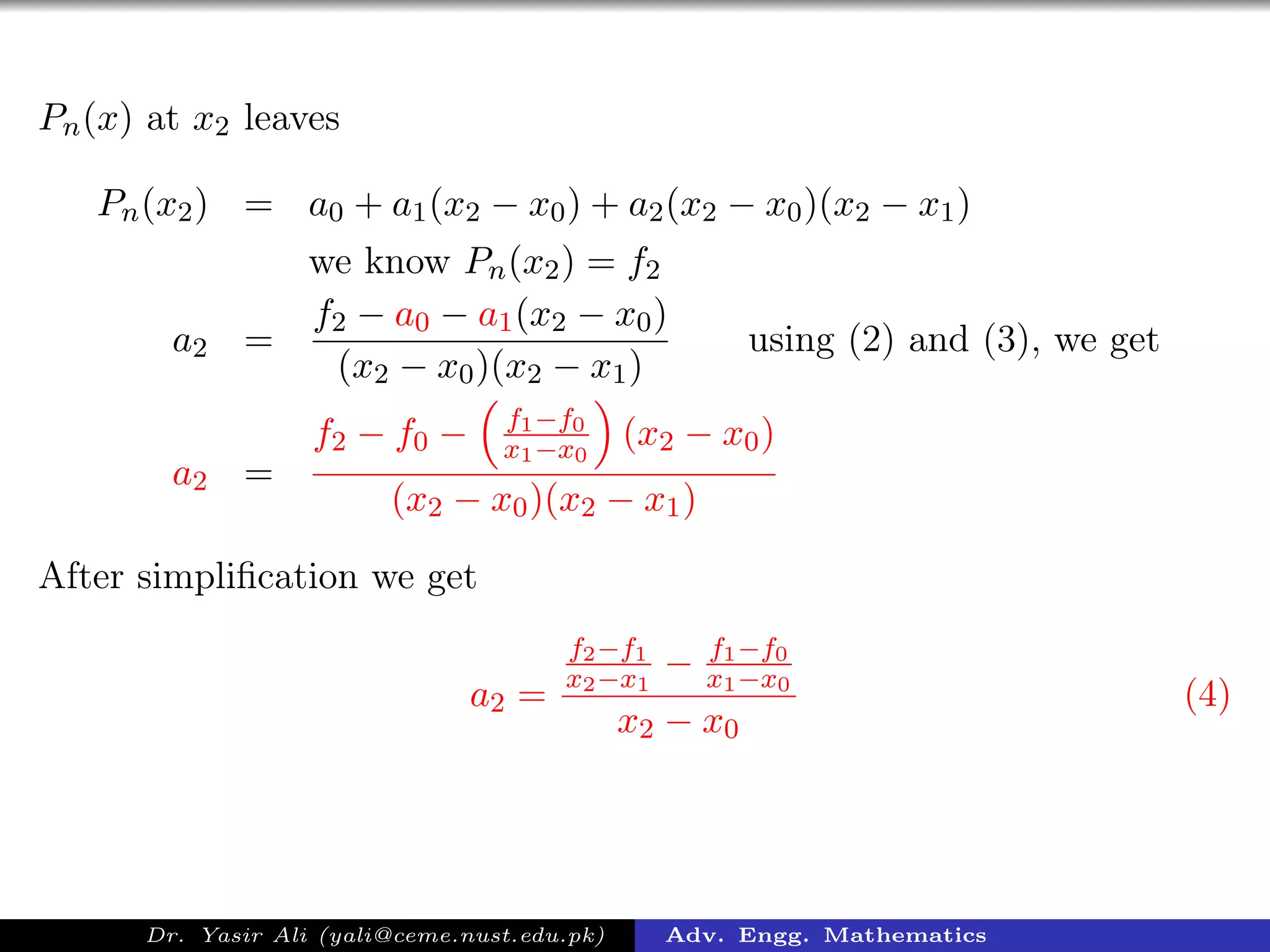
Hence, the interpolating polynomial (1) may be expressed as
Pn(x) = f[x0] + f[x1, x0](x − x0) + a2(x − x0)(x − x1)+
· · · + an(x − x0)(x − x1) · · · (x − xn),
where
ak = f[xk, xk−1, · · · , x1, x0] for k = 0, 1, · · · , n.
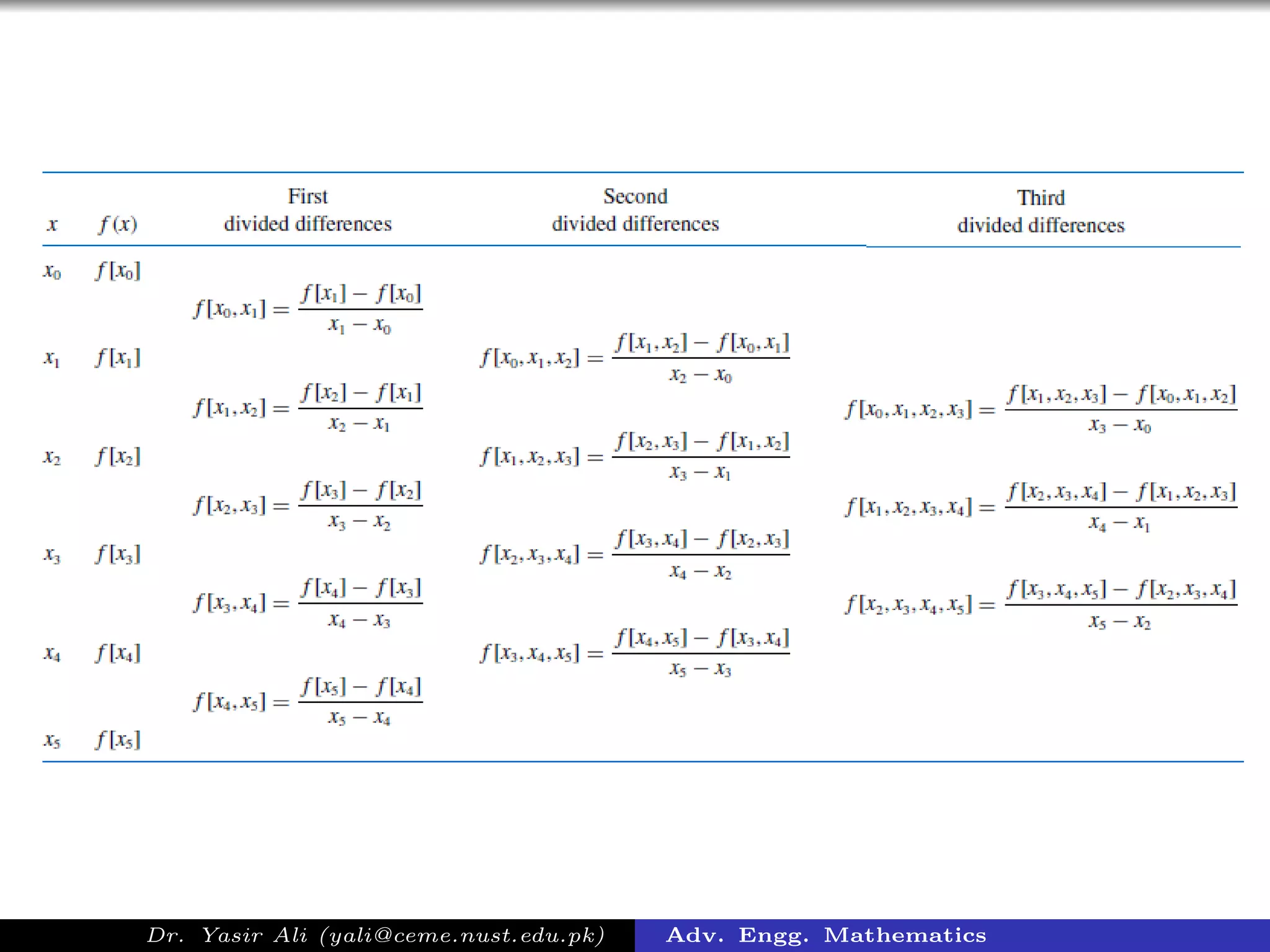
f[xi] = f(xi) zeroth divided difference
f[xi+1, xi] =
f[xi+1] − f[xi]
xi+1 − xi
1st divided difference
f[xi+2, xi+1, xi] =
f[xi+2, xi+1] − f[xi+1, xi]
xi+2 − xi
2nd divided difference
f[x0, x1, · · · , xk] =
Dr. Yasir Ali (yali@ceme.nust.edu.pk) Adv. Engg. Mathematics](https://image.slidesharecdn.com/812-i-dd-171231203845/75/Newtons-Divided-Difference-Formulation-18-2048.jpg)
![Newton’s Divided Difference
Hence, the interpolating polynomial (1) may be expressed as
Pn(x) = f[x0] + f[x1, x0](x − x0) + a2(x − x0)(x − x1)+
· · · + an(x − x0)(x − x1) · · · (x − xn),
where
ak = f[xk, xk−1, · · · , x1, x0] for k = 0, 1, · · · , n.
f[xi] = f(xi) zeroth divided difference
f[xi+1, xi] =
f[xi+1] − f[xi]
xi+1 − xi
1st divided difference
f[xi+2, xi+1, xi] =
f[xi+2, xi+1] − f[xi+1, xi]
xi+2 − xi
2nd divided difference
f[x0, x1, · · · , xk] =
f[xk, xk−1 · · · , x1] − f[xk−1, xk−2, · · · , x0]
xk − x0
Dr. Yasir Ali (yali@ceme.nust.edu.pk) Adv. Engg. Mathematics](https://image.slidesharecdn.com/812-i-dd-171231203845/75/Newtons-Divided-Difference-Formulation-19-2048.jpg)
![Complete the Divided Difference table for the following data
x 1.0 1.3 1.6 1.9 2.2
f(x) 0.7651 0.6201 0.4554 0.2818 0.1103
i xi f[xi] f[xi, xi−1] f[xi, xi−1, xi−2] f[xi, xi−1, xi−2, xi−3]
0 1.0 0.7651
♥
1 1.3 0.6201
2 1.6 0.4554
3 1.9 0.2818
4 2.2 0.1103
♥
Dr. Yasir Ali (yali@ceme.nust.edu.pk) Adv. Engg. Mathematics](https://image.slidesharecdn.com/812-i-dd-171231203845/75/Newtons-Divided-Difference-Formulation-21-2048.jpg)
![Complete the Divided Difference table for the following data
x 1.0 1.3 1.6 1.9 2.2
f(x) 0.7651 0.6201 0.4554 0.2818 0.1103
i xi f[xi] f[xi, xi−1] f[xi, xi−1, xi−2] f[xi, xi−1, xi−2, xi−3]
0 1.0 0.7651
♥
1 1.3 0.6201
2 1.6 0.4554
3 1.9 0.2818
4 2.2 0.1103
♥ The First Divided Difference involving x0 and x1 is
f[x0, x1] =
f[x1] − f[x0]
x1 − x0
=
0.6201 − 0.7651
1.3 − 1.0
= −0.4833.
Dr. Yasir Ali (yali@ceme.nust.edu.pk) Adv. Engg. Mathematics](https://image.slidesharecdn.com/812-i-dd-171231203845/75/Newtons-Divided-Difference-Formulation-22-2048.jpg)
![Complete the Divided Difference table for the following data
x 1.0 1.3 1.6 1.9 2.2
f(x) 0.7651 0.6201 0.4554 0.2818 0.1103
i xi f[xi] f[xi, xi−1] f[xi, xi−1, xi−2] f[xi, xi−1, xi−2, xi−3]
0 1.0 0.7651
♥
1 1.3 0.6201
2 1.6 0.4554
3 1.9 0.2818
4 2.2 0.1103
♥ The First Divided Difference involving x0 and x1 is
f[x0, x1] =
f[x1] − f[x0]
x1 − x0
=
0.6201 − 0.7651
1.3 − 1.0
= −0.4833.
Remaining First Divided Differences are as follows
Dr. Yasir Ali (yali@ceme.nust.edu.pk) Adv. Engg. Mathematics](https://image.slidesharecdn.com/812-i-dd-171231203845/75/Newtons-Divided-Difference-Formulation-23-2048.jpg)
![Complete the Divided Difference table for the following data
x 1.0 1.3 1.6 1.9 2.2
f(x) 0.7651 0.6201 0.4554 0.2818 0.1103
i xi f[xi] f[xi, xi−1] f[xi, xi−1, xi−2] f[xi, xi−1, xi−2, xi−3]
0 1.0 0.7651
-0.4833
1 1.3 0.6201 ♠
-0.549
2 1.6 0.4554
-0.5787
3 1.9 0.2818
-0.5717
4 2.2 0.1103
♠
Dr. Yasir Ali (yali@ceme.nust.edu.pk) Adv. Engg. Mathematics](https://image.slidesharecdn.com/812-i-dd-171231203845/75/Newtons-Divided-Difference-Formulation-24-2048.jpg)
![Complete the Divided Difference table for the following data
x 1.0 1.3 1.6 1.9 2.2
f(x) 0.7651 0.6201 0.4554 0.2818 0.1103
i xi f[xi] f[xi, xi−1] f[xi, xi−1, xi−2] f[xi, xi−1, xi−2, xi−3]
0 1.0 0.7651
-0.4833
1 1.3 0.6201 ♠
-0.549
2 1.6 0.4554
-0.5787
3 1.9 0.2818
-0.5717
4 2.2 0.1103
♠The Second Divided Difference involving x0, x1 and x2 is
f[x2, x1, x0] =
f[x2, x1] − f[x1, x0]
x2 − x0
=
−0.549 − (−0.4833)
1.6 − 1.0
= −0.1094
Dr. Yasir Ali (yali@ceme.nust.edu.pk) Adv. Engg. Mathematics](https://image.slidesharecdn.com/812-i-dd-171231203845/75/Newtons-Divided-Difference-Formulation-25-2048.jpg)
![Complete the Divided Difference table for the following data
x 1.0 1.3 1.6 1.9 2.2
f(x) 0.7651 0.6201 0.4554 0.2818 0.1103
i xi f[xi] f[xi, xi−1] f[xi, xi−1, xi−2] f[xi, xi−1, xi−2, xi−3]
0 1.0 0.7651
-0.4833
1 1.3 0.6201 ♠
-0.549
2 1.6 0.4554
-0.5787
3 1.9 0.2818
-0.5717
4 2.2 0.1103
♠The Second Divided Difference involving x0, x1 and x2 is
f[x2, x1, x0] =
f[x2, x1] − f[x1, x0]
x2 − x0
=
−0.549 − (−0.4833)
1.6 − 1.0
= −0.1094
Remaining Second Divided Difference are as follows
Dr. Yasir Ali (yali@ceme.nust.edu.pk) Adv. Engg. Mathematics](https://image.slidesharecdn.com/812-i-dd-171231203845/75/Newtons-Divided-Difference-Formulation-26-2048.jpg)
![Complete the Divided Difference table for the following data
x 1.0 1.3 1.6 1.9 2.2
f(x) 0.7651 0.6201 0.4554 0.2818 0.1103
i xi f[xi] f[xi, xi−1] f[xi, xi−1, xi−2] f[xi, xi−1, xi−2, xi−3]
0 1.0 0.7651
-0.4833
1 1.3 0.6201 -0.1094
-0.549 ♣
2 1.6 0.4554 -0.0494
-0.5787
3 1.9 0.2818 0.0117
-0.5717
4 2.2 0.1103
♣
Dr. Yasir Ali (yali@ceme.nust.edu.pk) Adv. Engg. Mathematics](https://image.slidesharecdn.com/812-i-dd-171231203845/75/Newtons-Divided-Difference-Formulation-27-2048.jpg)
![Complete the Divided Difference table for the following data
x 1.0 1.3 1.6 1.9 2.2
f(x) 0.7651 0.6201 0.4554 0.2818 0.1103
i xi f[xi] f[xi, xi−1] f[xi, xi−1, xi−2] f[xi, xi−1, xi−2, xi−3]
0 1.0 0.7651
-0.4833
1 1.3 0.6201 -0.1094
-0.549 ♣
2 1.6 0.4554 -0.0494
-0.5787
3 1.9 0.2818 0.0117
-0.5717
4 2.2 0.1103
♣The Third Divided Difference f[x3, x2, x1, x0]
=
f[x3, x2, x1] − f[x2, x1, x0]
x3 − x0
=
−0.1094 − (−0.494)
1.9 − 1.0
= −0.0667
Dr. Yasir Ali (yali@ceme.nust.edu.pk) Adv. Engg. Mathematics](https://image.slidesharecdn.com/812-i-dd-171231203845/75/Newtons-Divided-Difference-Formulation-28-2048.jpg)
![Complete the Divided Difference table for the following data
x 1.0 1.3 1.6 1.9 2.2
f(x) 0.7651 0.6201 0.4554 0.2818 0.1103
i xi f[xi] f[xi, xi−1] f[xi, xi−1, xi−2] f[xi, xi−1, xi−2, xi−3]
0 1.0 0.7651
-0.4833
1 1.3 0.6201 -0.1094
-0.549 ♣
2 1.6 0.4554 -0.0494
-0.5787
3 1.9 0.2818 0.0117
-0.5717
4 2.2 0.1103
♣The Third Divided Difference f[x3, x2, x1, x0]
=
f[x3, x2, x1] − f[x2, x1, x0]
x3 − x0
=
−0.1094 − (−0.494)
1.9 − 1.0
= −0.0667
Remaining Third Divided Differences are as follows
Dr. Yasir Ali (yali@ceme.nust.edu.pk) Adv. Engg. Mathematics](https://image.slidesharecdn.com/812-i-dd-171231203845/75/Newtons-Divided-Difference-Formulation-29-2048.jpg)
![Complete the Divided Difference table for the following data
x 1.0 1.3 1.6 1.9 2.2
f(x) 0.7651 0.6201 0.4554 0.2818 0.1103
i xi f[xi] f[xi, xi−1] f[xi, xi−1, xi−2] f[xi, xi−1, xi−2, xi−3]
0 1.0 0.7651
-0.4833
1 1.3 0.6201 -0.1094
-0.549 -0.0667
2 1.6 0.4554 -0.0494
-0.5787 0.0679
3 1.9 0.2818 0.0117
-0.5717
4 2.2 0.1103
Dr. Yasir Ali (yali@ceme.nust.edu.pk) Adv. Engg. Mathematics](https://image.slidesharecdn.com/812-i-dd-171231203845/75/Newtons-Divided-Difference-Formulation-30-2048.jpg)
![Complete the Divided Difference table for the following data
x 1.0 1.3 1.6 1.9 2.2
f(x) 0.7651 0.6201 0.4554 0.2818 0.1103
i xi f[xi] f[xi, xi−1] f[xi, xi−1, xi−2] f[xi, xi−1, xi−2, xi−3]
0 1.0 0.7651
-0.4833
1 1.3 0.6201 -0.1094
-0.549 -0.0667
2 1.6 0.4554 -0.0494
-0.5787 0.0679
3 1.9 0.2818 0.0117
-0.5717
4 2.2 0.1103
The Fourth Divided Difference f[x4, x3, x2, x1, x0]
=
f[x4, x3, x2, x1] − f[x3, x2, x1, x0]
x3 − x0
=
−0.0679 − (−0.0667)
2.2 − 1.0
= −0.001
Dr. Yasir Ali (yali@ceme.nust.edu.pk) Adv. Engg. Mathematics](https://image.slidesharecdn.com/812-i-dd-171231203845/75/Newtons-Divided-Difference-Formulation-31-2048.jpg)
![Complete the Divided Difference table for the following data
x 1.0 1.3 1.6 1.9 2.2
f(x) 0.7651 0.6201 0.4554 0.2818 0.1103
i xi f[xi] f[xi, xi−1] f[xi, xi−1, xi−2] f[xi, xi−1, xi−2, xi−3]
0 1.0 0.7651
-0.4833
1 1.3 0.6201 -0.1094
-0.549 -0.0667
2 1.6 0.4554 -0.0494
-0.5787 0.0679
3 1.9 0.2818 0.0117
-0.5717
4 2.2 0.1103
The Fourth Divided Difference f[x4, x3, x2, x1, x0]
=
f[x4, x3, x2, x1] − f[x3, x2, x1, x0]
x3 − x0
=
−0.0679 − (−0.0667)
2.2 − 1.0
= −0.001
This would be last divided difference in this case.
Dr. Yasir Ali (yali@ceme.nust.edu.pk) Adv. Engg. Mathematics](https://image.slidesharecdn.com/812-i-dd-171231203845/75/Newtons-Divided-Difference-Formulation-32-2048.jpg)
![The coefficients of the Newton forward divided-difference form of the
interpolating polynomial are along the diagonal in the table. This
polynomial is
P4(x) = 0.7651 − 0.4833(x − 1) − 1094(x − 1)(x − 1.3)+
−0667(x − 1)(x − 1.3)(x − 1.6) − 0.001(x − 1)(x − 1.3)(x − 1.6)(x − 1.9)
i xi f[xi] f[xi, xi−1] f[xi, xi−1, xi−2] f[xi, xi−1, xi−2, xi−3]
0 1.0 0.7651
-0.4833
1 1.3 0.6201 -0.1094
-0.549 -0.0667
2 1.6 0.4554 -0.0494
-0.5787 0.0679
3 1.9 0.2818 0.0117
-0.5717
4 2.2 0.1103
Dr. Yasir Ali (yali@ceme.nust.edu.pk) Adv. Engg. Mathematics](https://image.slidesharecdn.com/812-i-dd-171231203845/75/Newtons-Divided-Difference-Formulation-33-2048.jpg)
![The coefficients of the Newton forward divided-difference form of the
interpolating polynomial are along the diagonal in the table. This
polynomial is
P4(x) = 0.7651 − 0.4833(x − 1) − 1094(x − 1)(x − 1.3)+
−0667(x − 1)(x − 1.3)(x − 1.6) − 0.001(x − 1)(x − 1.3)(x − 1.6)(x − 1.9)
i xi f[xi] f[xi, xi−1] f[xi, xi−1, xi−2] f[xi, xi−1, xi−2, xi−3]
0 1.0 0.7651
-0.4833
1 1.3 0.6201 -0.1094
-0.549 -0.0667
2 1.6 0.4554 -0.0494
-0.5787 0.0679
3 1.9 0.2818 0.0117
-0.5717
4 2.2 0.1103
f[x4, x3, x2, x1, x0] = −0.001
Dr. Yasir Ali (yali@ceme.nust.edu.pk) Adv. Engg. Mathematics](https://image.slidesharecdn.com/812-i-dd-171231203845/75/Newtons-Divided-Difference-Formulation-34-2048.jpg)
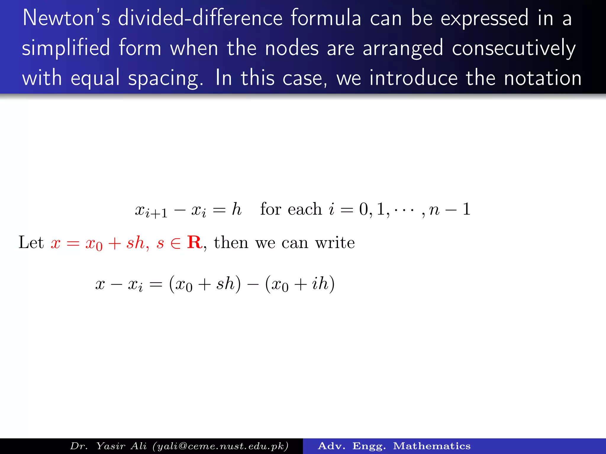
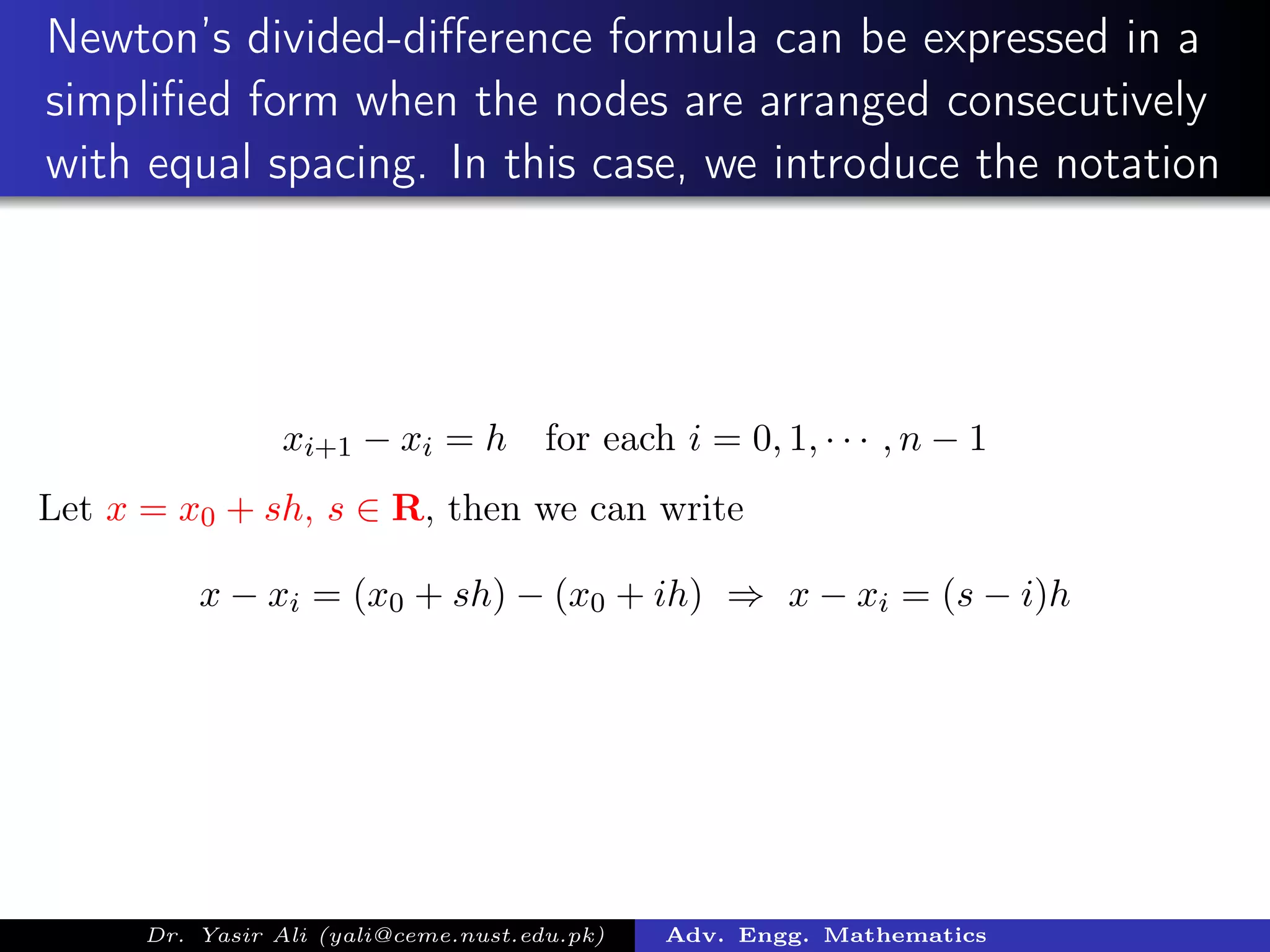
![Using x − xi = (s − i)h in
Pn(x) = f[x0] + f[x1, x0](x − x0) + a2(x − x0)(x − x1)+
· · · + an(x − x0)(x − x1) · · · (x − xn),
where
ak = f[xk, xk−1, · · · , x1, x0] for k = 0, 1, · · · , n.
We obtain
Dr. Yasir Ali (yali@ceme.nust.edu.pk) Adv. Engg. Mathematics](https://image.slidesharecdn.com/812-i-dd-171231203845/75/Newtons-Divided-Difference-Formulation-37-2048.jpg)
![Using x − xi = (s − i)h in
Pn(x) = f[x0] + f[x1, x0](x − x0) + a2(x − x0)(x − x1)+
· · · + an(x − x0)(x − x1) · · · (x − xn),
where
ak = f[xk, xk−1, · · · , x1, x0] for k = 0, 1, · · · , n.
We obtain
Pn(x) = Pn(x0 + sh) = f[x0] + shf[x1, x0] + s(s − 1)h2
f[x2, x1, x0]+
s(s − 1)(s − 2)h3
f[x3, x2, x1, x0] + · · · +
+s(s − 1)(s − 2) · · · (s − n + 1)hn
f[xn, xn−1, · · · , x0]
Dr. Yasir Ali (yali@ceme.nust.edu.pk) Adv. Engg. Mathematics](https://image.slidesharecdn.com/812-i-dd-171231203845/75/Newtons-Divided-Difference-Formulation-38-2048.jpg)
![Using x − xi = (s − i)h in
Pn(x) = f[x0] + f[x1, x0](x − x0) + a2(x − x0)(x − x1)+
· · · + an(x − x0)(x − x1) · · · (x − xn),
where
ak = f[xk, xk−1, · · · , x1, x0] for k = 0, 1, · · · , n.
We obtain
Pn(x) = Pn(x0 + sh) = f[x0] + shf[x1, x0] + s(s − 1)h2
f[x2, x1, x0]+
s(s − 1)(s − 2)h3
f[x3, x2, x1, x0] + · · · +
+s(s − 1)(s − 2) · · · (s − n + 1)hn
f[xn, xn−1, · · · , x0]
Note that
x − x0 = sh
x − x1 = (s − 1)h & x − x0 = sh ⇒
Dr. Yasir Ali (yali@ceme.nust.edu.pk) Adv. Engg. Mathematics](https://image.slidesharecdn.com/812-i-dd-171231203845/75/Newtons-Divided-Difference-Formulation-39-2048.jpg)
![Using x − xi = (s − i)h in
Pn(x) = f[x0] + f[x1, x0](x − x0) + a2(x − x0)(x − x1)+
· · · + an(x − x0)(x − x1) · · · (x − xn),
where
ak = f[xk, xk−1, · · · , x1, x0] for k = 0, 1, · · · , n.
We obtain
Pn(x) = Pn(x0 + sh) = f[x0] + shf[x1, x0] + s(s − 1)h2
f[x2, x1, x0]+
s(s − 1)(s − 2)h3
f[x3, x2, x1, x0] + · · · +
+s(s − 1)(s − 2) · · · (s − n + 1)hn
f[xn, xn−1, · · · , x0]
Note that
x − x0 = sh
x − x1 = (s − 1)h & x − x0 = sh ⇒ (x − x1)(x − x0) = s(s − 1)h2
similarly (x − x0)(x − x1)(x − x2) = s(s − 1)(s − 2)h3
Dr. Yasir Ali (yali@ceme.nust.edu.pk) Adv. Engg. Mathematics](https://image.slidesharecdn.com/812-i-dd-171231203845/75/Newtons-Divided-Difference-Formulation-40-2048.jpg)
![Equi-spaced Divided Difference
Pn(x0 + sh) = f[x0] +
n
k=1
s(s − 1) · · · (s − k + 1)hk
f[xk, xk−1, · · · , x0]
Using binomial-coefficient notation,
s
k
=
s(s − 1) · · · (s − k + 1)
k!
Dr. Yasir Ali (yali@ceme.nust.edu.pk) Adv. Engg. Mathematics](https://image.slidesharecdn.com/812-i-dd-171231203845/75/Newtons-Divided-Difference-Formulation-41-2048.jpg)
![Equi-spaced Divided Difference
Pn(x0 + sh) = f[x0] +
n
k=1
s(s − 1) · · · (s − k + 1)hk
f[xk, xk−1, · · · , x0]
Using binomial-coefficient notation,
s
k
=
s(s − 1) · · · (s − k + 1)
k!
⇒ s(s−1) · · · (s−k +1) = k!
s
k
.
Dr. Yasir Ali (yali@ceme.nust.edu.pk) Adv. Engg. Mathematics](https://image.slidesharecdn.com/812-i-dd-171231203845/75/Newtons-Divided-Difference-Formulation-42-2048.jpg)
![Equi-spaced Divided Difference
Pn(x0 + sh) = f[x0] +
n
k=1
s(s − 1) · · · (s − k + 1)hk
f[xk, xk−1, · · · , x0]
Using binomial-coefficient notation,
s
k
=
s(s − 1) · · · (s − k + 1)
k!
⇒ s(s−1) · · · (s−k +1) = k!
s
k
.
Thus we can express Pn(x) compactly as
Pn(x) = Pn(x0 + sh) = f[x0] +
n
k=1
k!
s
k
hk
f[xk, xk−1, · · · , x0]
Dr. Yasir Ali (yali@ceme.nust.edu.pk) Adv. Engg. Mathematics](https://image.slidesharecdn.com/812-i-dd-171231203845/75/Newtons-Divided-Difference-Formulation-43-2048.jpg)
![Newton forward-difference formula
The Newton forward-difference formula, is constructed by making use
of the forward difference notation ∆. With this notation,
f[x1, x0] =
f[x1] − f[x0]
x1 − x0
=
1
h
(f(x1) − f(x0)) =
1
h
∆f(x0)
Similarly
f[x2, x1, x0] =
f[x2, x1] − f[x1, x0]
x2 − x0
=
1
2h
(f[x2, x1] − f[x1, x0])
=
1
2h
1
h
(∆f(x1) − ∆f(x0))
=
1
2h2
(∆(f(x1) − f(x0)))
=
1
2h2
(∆(∆f(x0))) =
Dr. Yasir Ali (yali@ceme.nust.edu.pk) Adv. Engg. Mathematics](https://image.slidesharecdn.com/812-i-dd-171231203845/75/Newtons-Divided-Difference-Formulation-44-2048.jpg)
![Newton forward-difference formula
The Newton forward-difference formula, is constructed by making use
of the forward difference notation ∆. With this notation,
f[x1, x0] =
f[x1] − f[x0]
x1 − x0
=
1
h
(f(x1) − f(x0)) =
1
h
∆f(x0)
Similarly
f[x2, x1, x0] =
f[x2, x1] − f[x1, x0]
x2 − x0
=
1
2h
(f[x2, x1] − f[x1, x0])
=
1
2h
1
h
(∆f(x1) − ∆f(x0))
=
1
2h2
(∆(f(x1) − f(x0)))
=
1
2h2
(∆(∆f(x0))) =
1
2h2
∆2
f(x0)
Dr. Yasir Ali (yali@ceme.nust.edu.pk) Adv. Engg. Mathematics](https://image.slidesharecdn.com/812-i-dd-171231203845/75/Newtons-Divided-Difference-Formulation-45-2048.jpg)
![Newton forward-difference formula
Note that
f[x1, x0] =
1
h
∆f(x0)
f[x2, x1, x0] =
1
2h2
∆2
f(x0)
In general
f[xk, xk−1, · · · , x0] =
1
k!hk
∆k
f(x0)
Pn(x) = Pn(x0 + sh) = f[x0] +
n
k=1
k!
s
k
hk
f[xk, xk−1, · · · , x0]
Pn(x) = Pn(x0 + sh) = f(x0) +
n
k=1
s
k
∆k
f(x0)
Dr. Yasir Ali (yali@ceme.nust.edu.pk) Adv. Engg. Mathematics](https://image.slidesharecdn.com/812-i-dd-171231203845/75/Newtons-Divided-Difference-Formulation-46-2048.jpg)


The document discusses Lagrange interpolation and divided differences. It explains that the Lagrange interpolation polynomial can be written in terms of divided differences, where the coefficients are divided differences of the function values. Divided differences are defined recursively, and a pattern is identified to write them in terms of the function values at nodes. An example divided difference table is given for a set of data points.
Introduction to Advanced Engineering Mathematics and focus on divided differences interpolations.
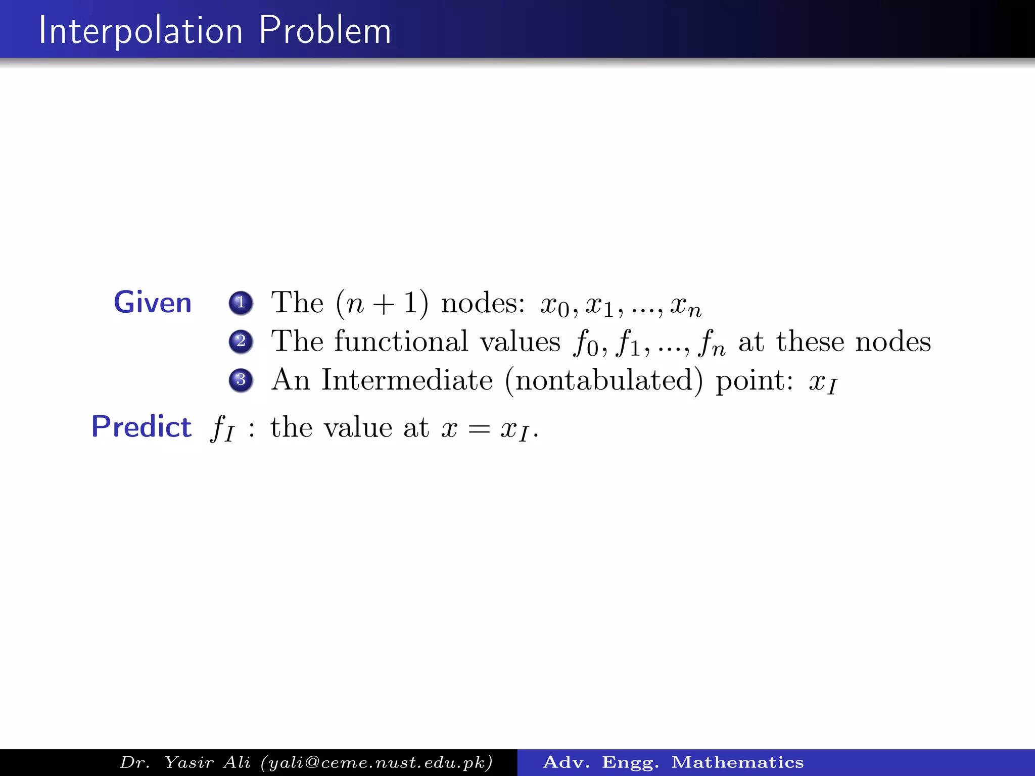
Defines the interpolation problem with n+1 nodes and corresponding functional values to predict an intermediate value.
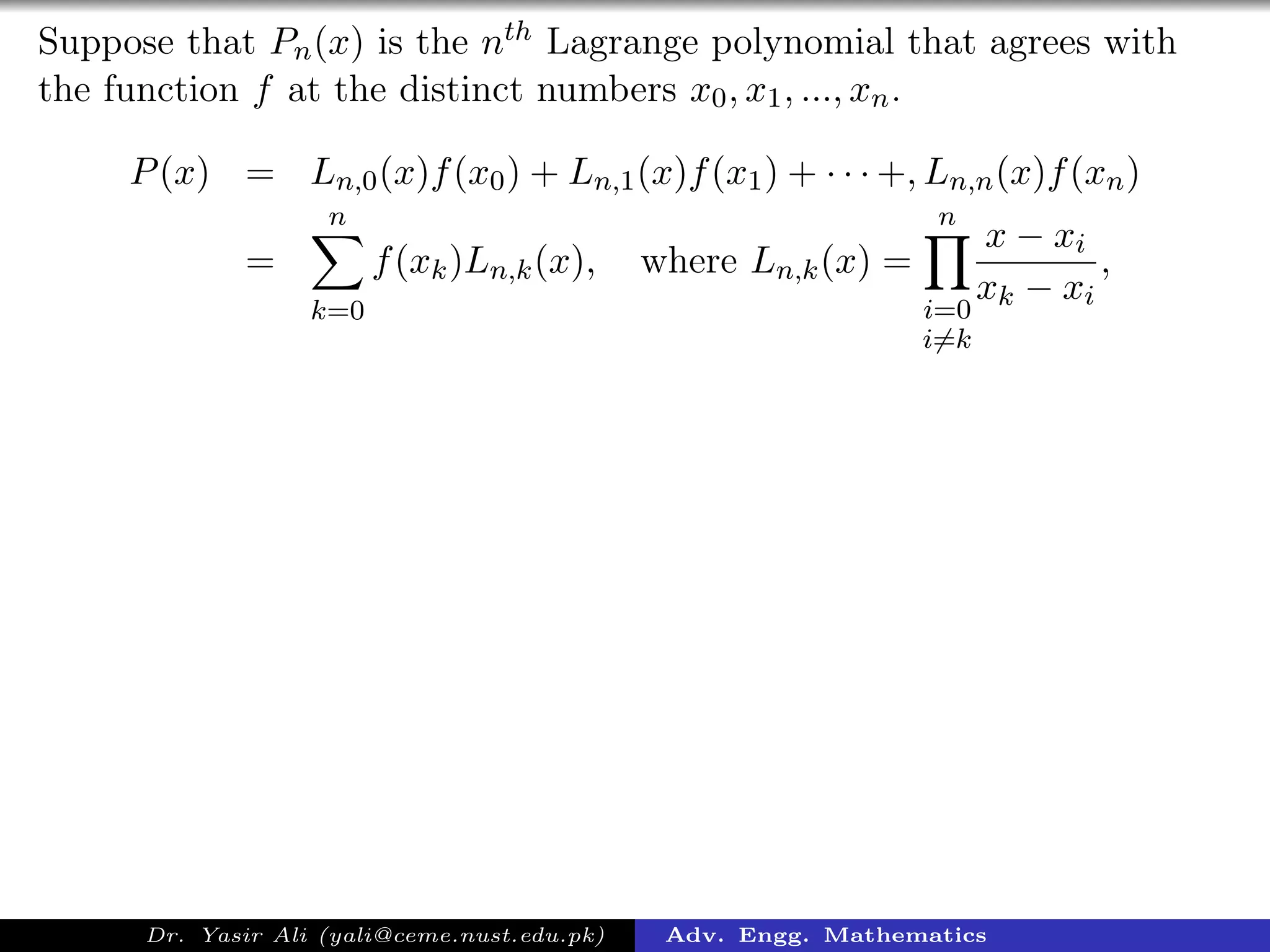
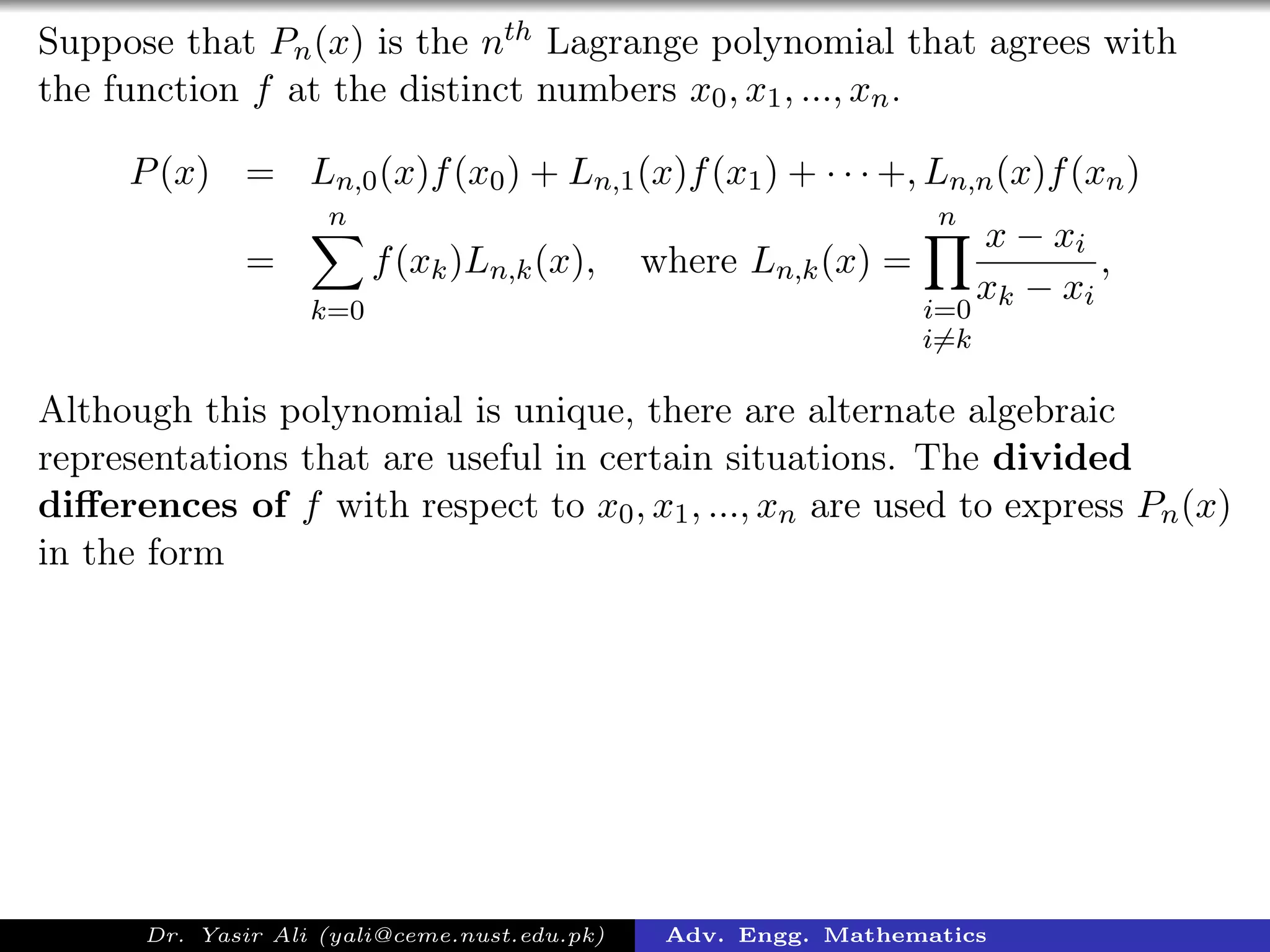
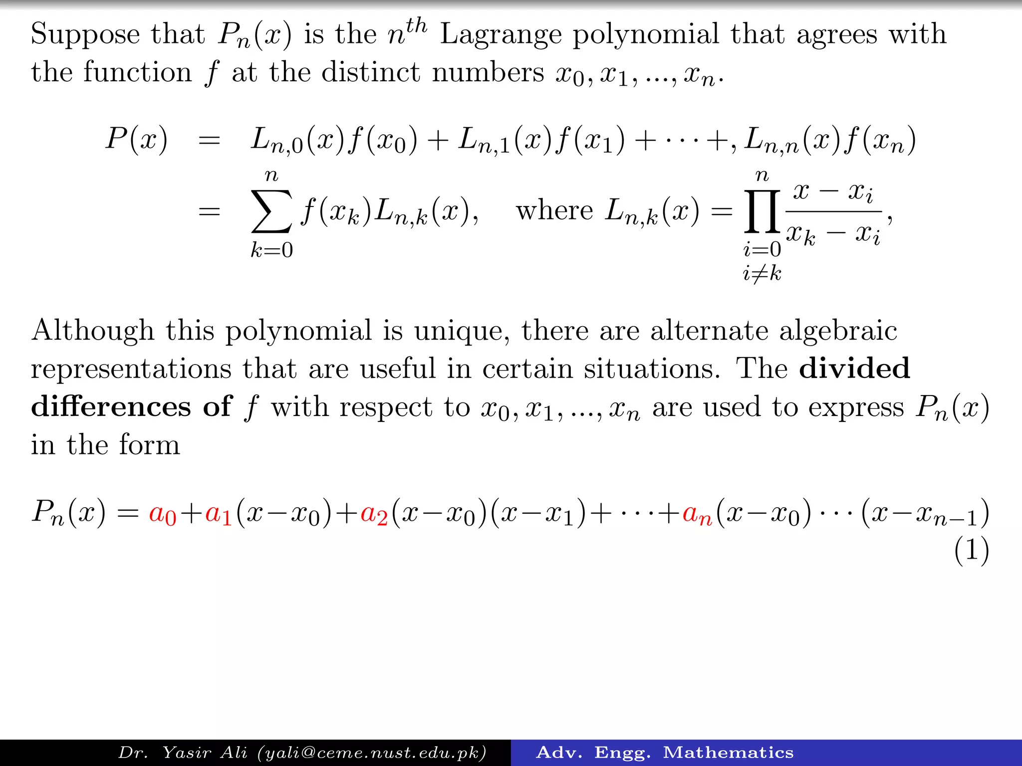
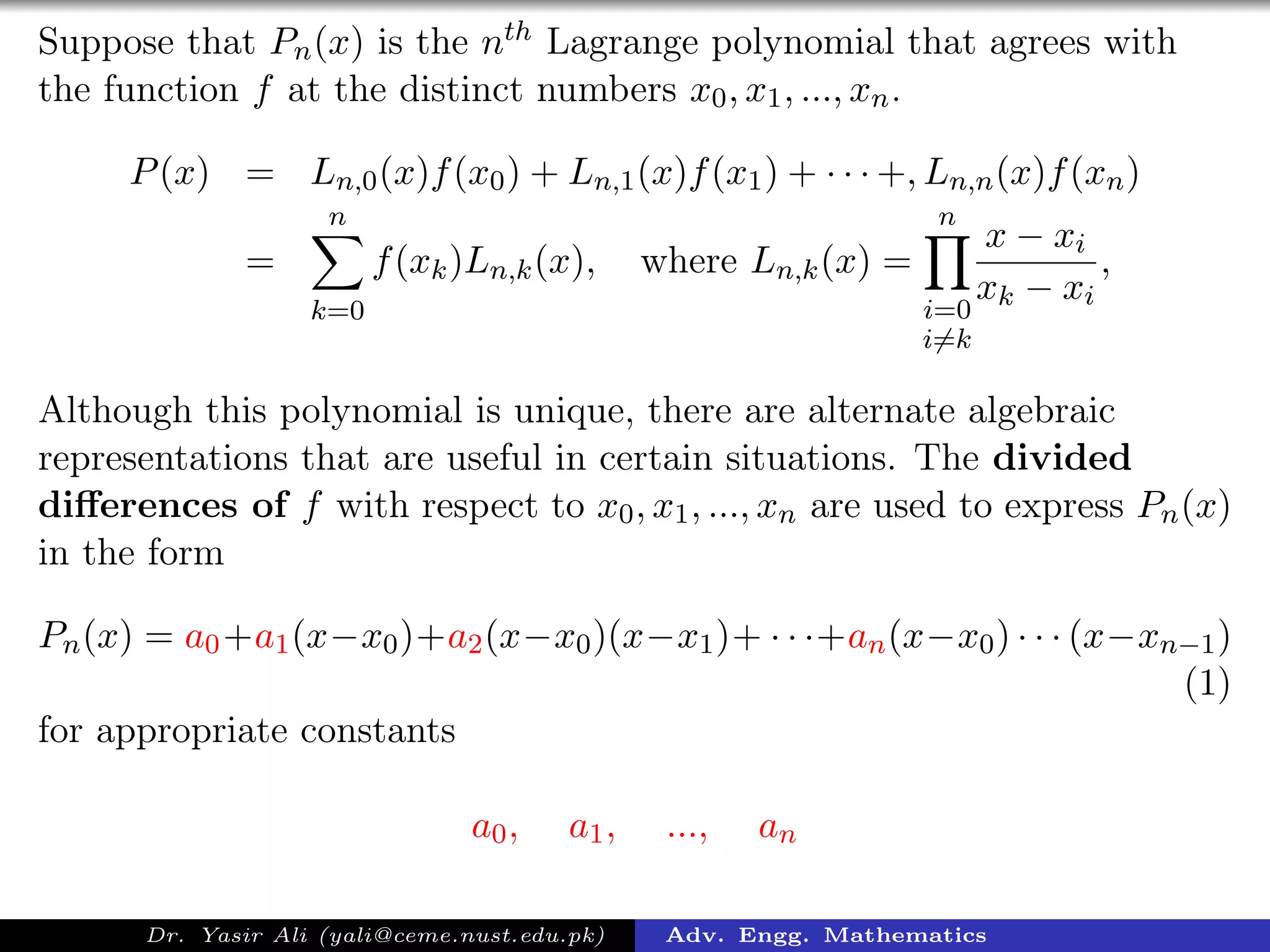
Introduces the nth Lagrange polynomial for interpolation and discusses alternative forms using divided differences.
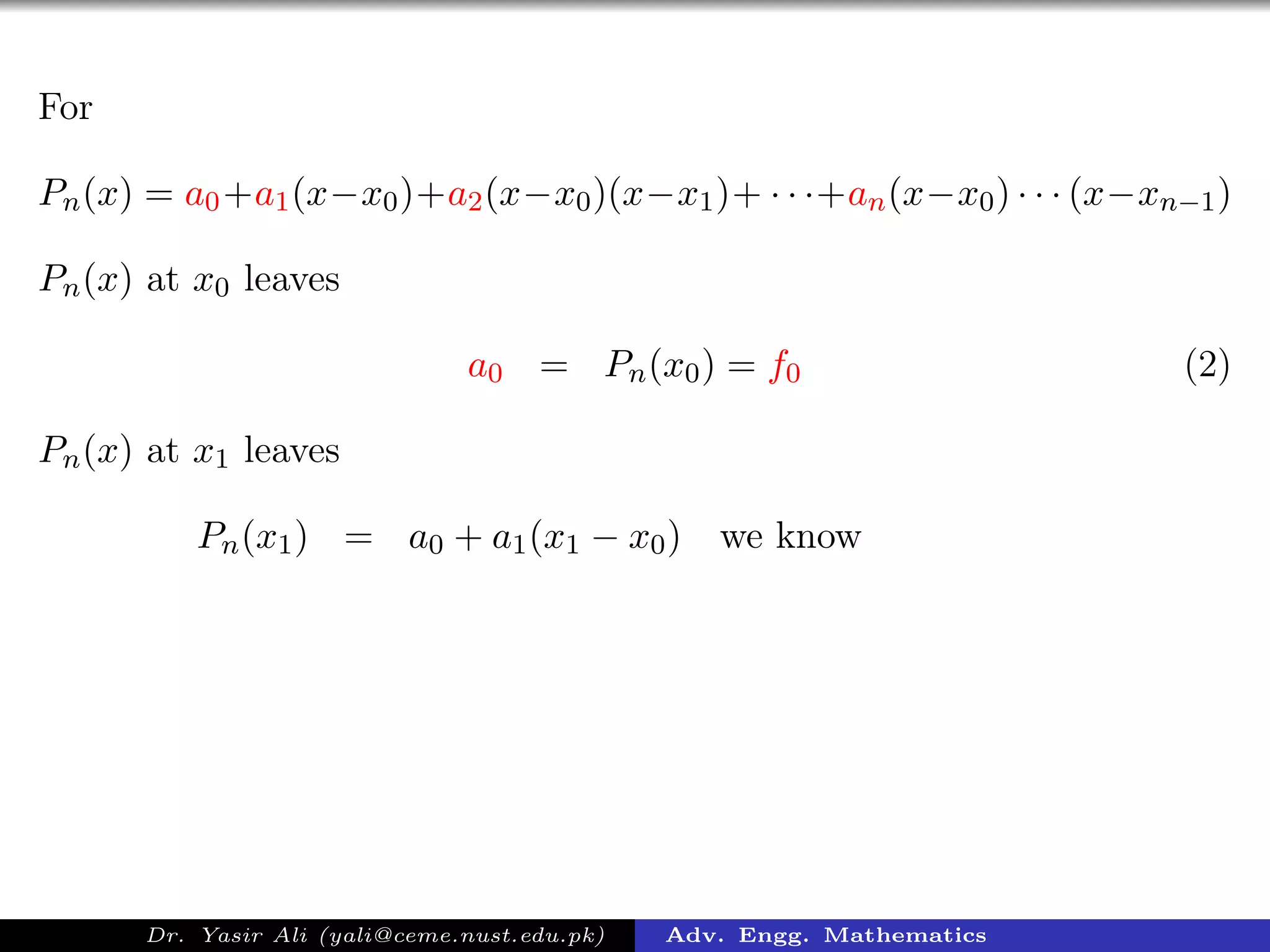
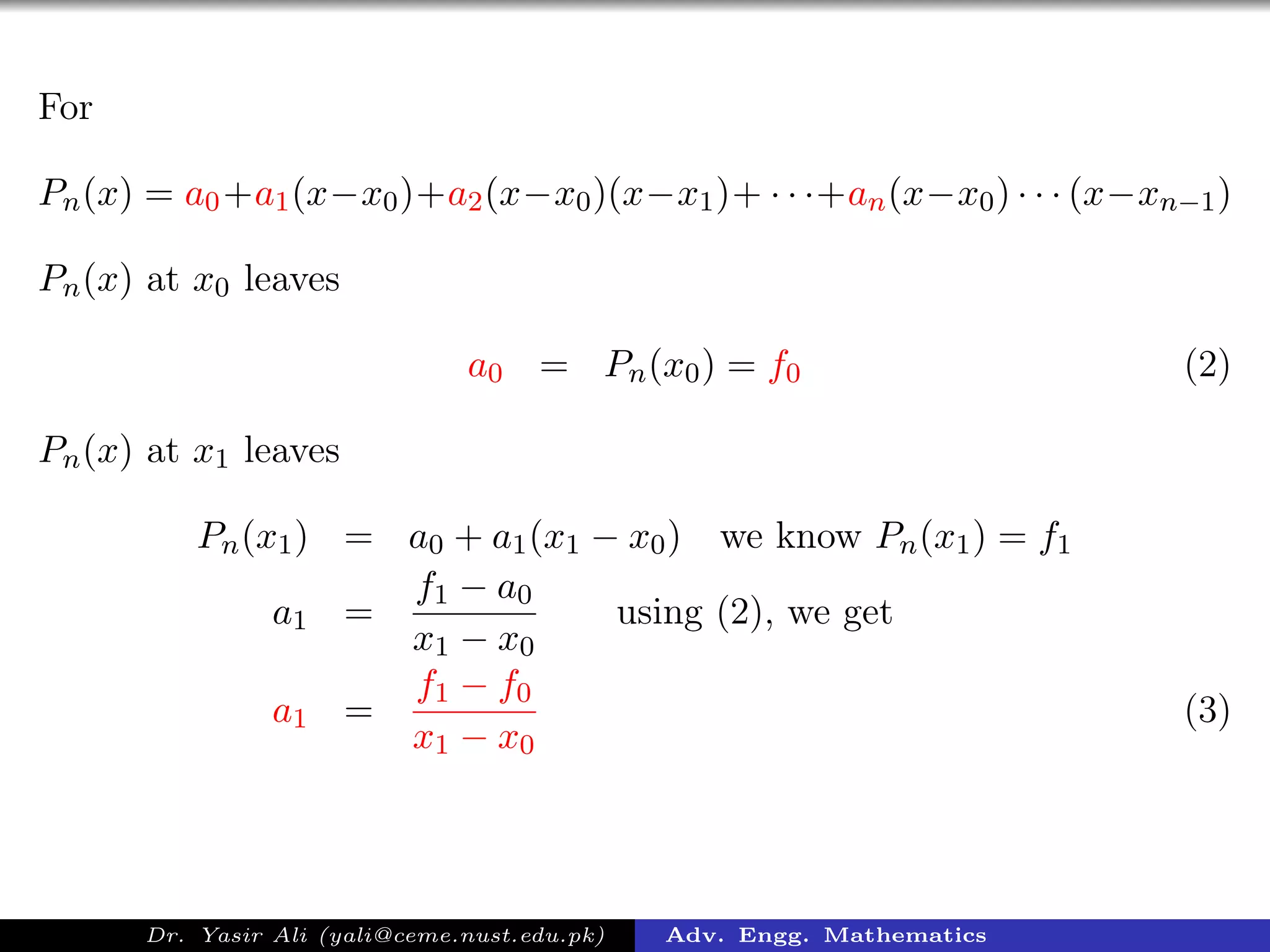
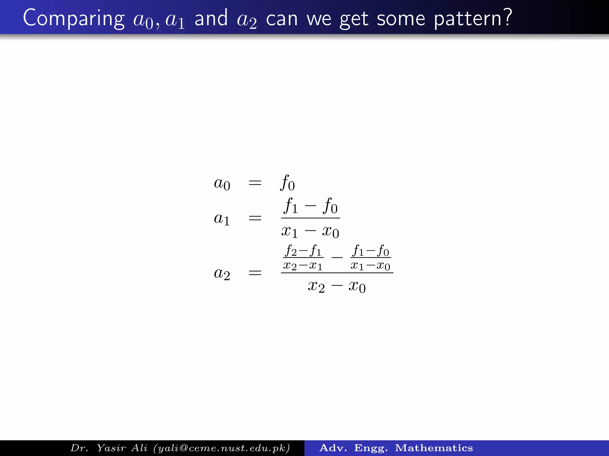
Explains how coefficients a0, a1, and a2 are derived from functional values and form the basis for constructing the polynomial.
Explores the pattern in coefficients leading to the formulation of higher order coefficients using divided differences.
Introduces Newton’s divided difference representation for deriving the interpolating polynomial based on divided differences.
Provides a hands-on example of completing a divided difference table with specific values to illustrate the technique.
Explains how to simplify Newton’s divided difference formula with equal spacing between nodes for computations.
Demonstrates employing binomial coefficients in equi-spaced divided differences for constructing interpolating polynomials.
Introduces and formulates Newton forward-difference using the forward difference notation to derive values functionally.
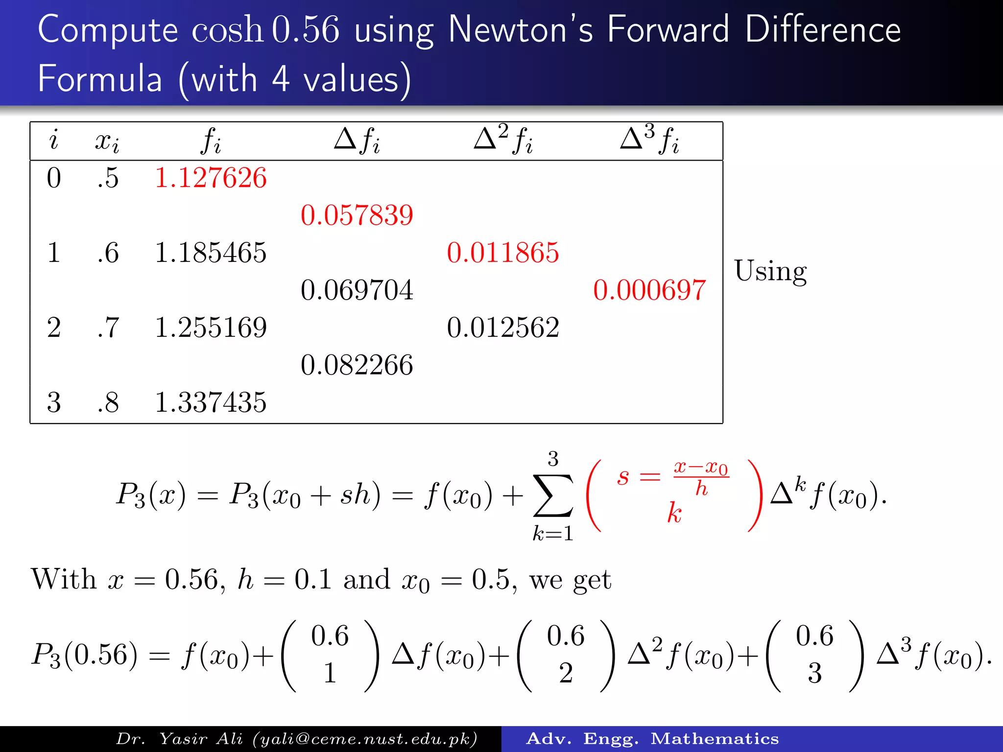
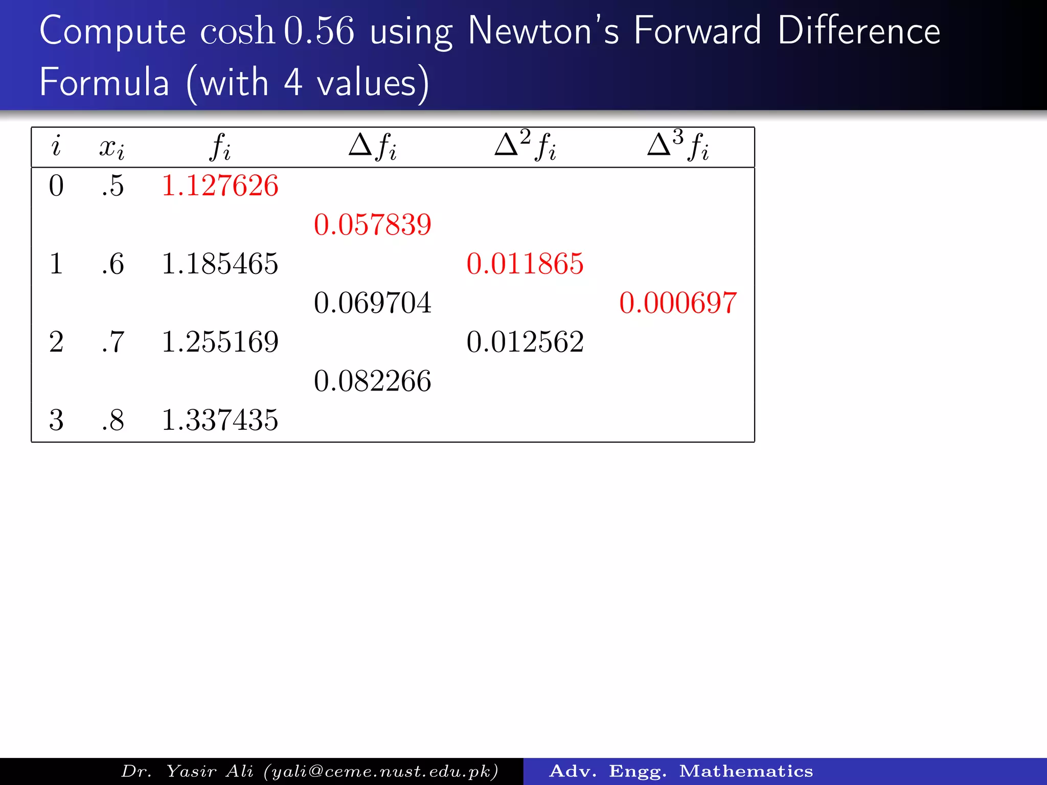
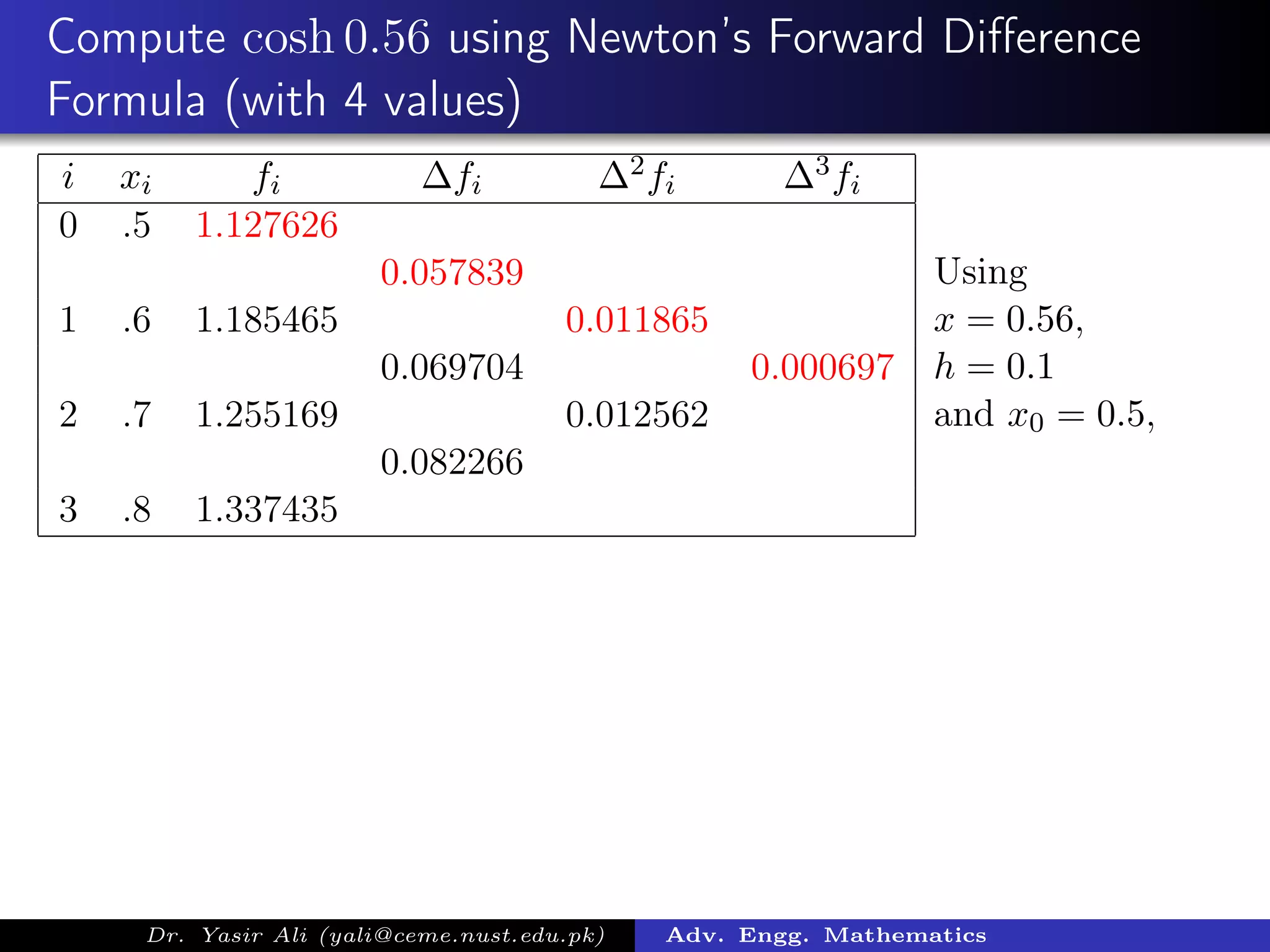
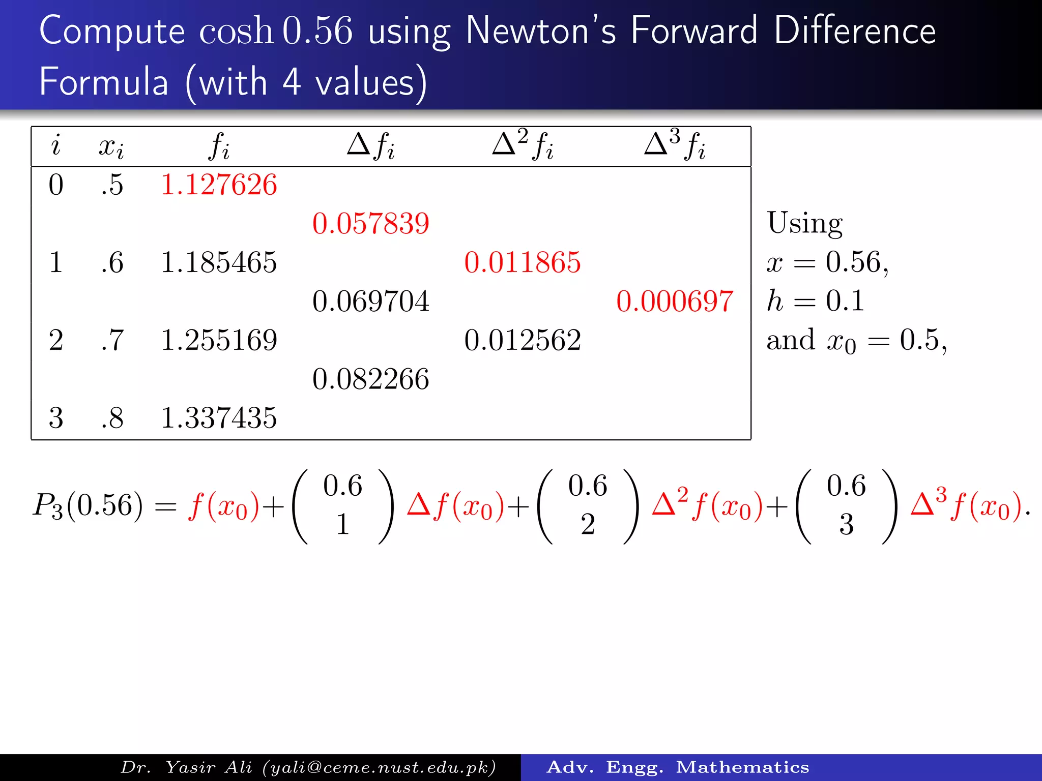
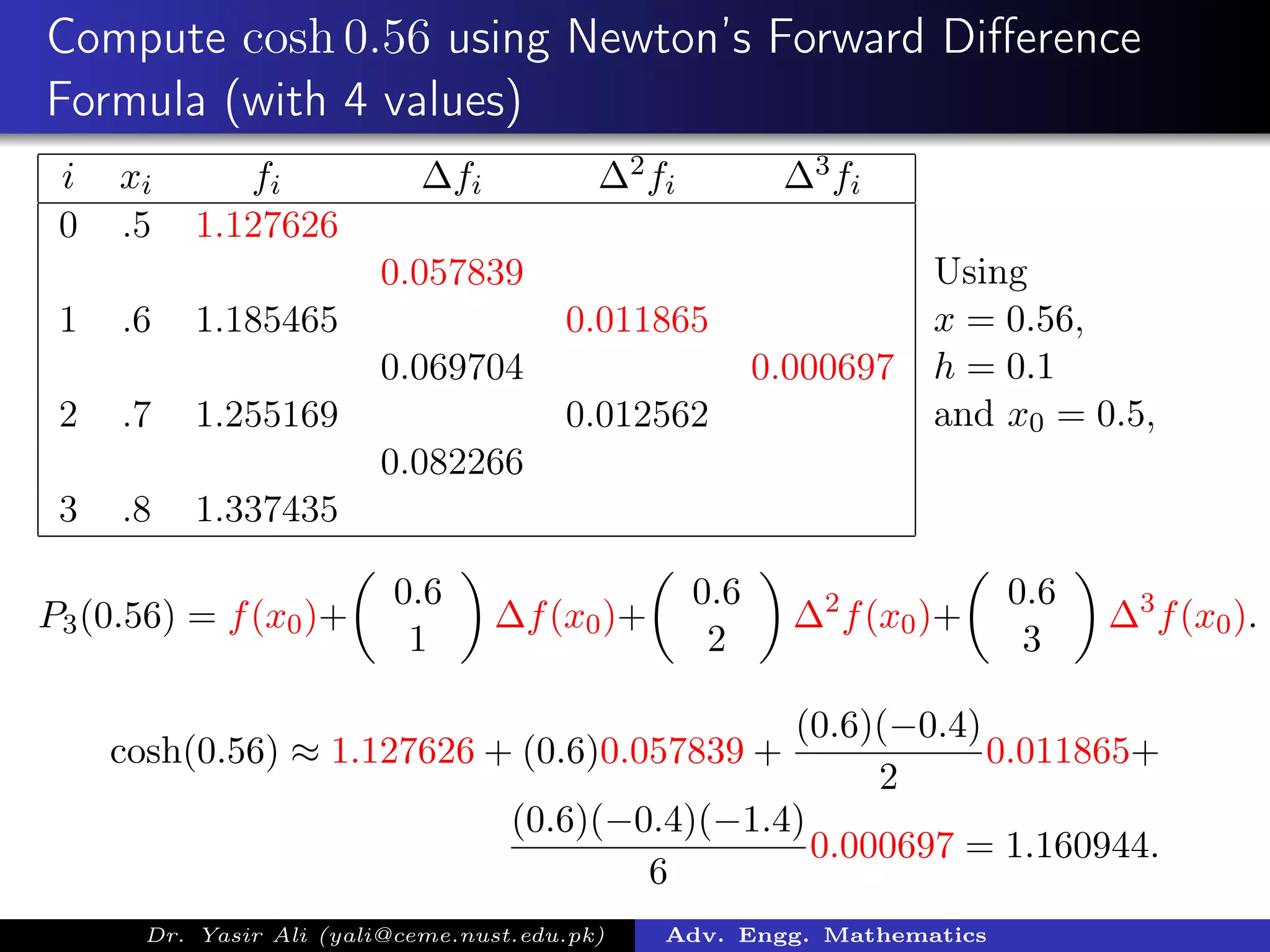
Illustrates the application of Newton’s forward difference formula in computing values such as cosh(0.56) using sample data.
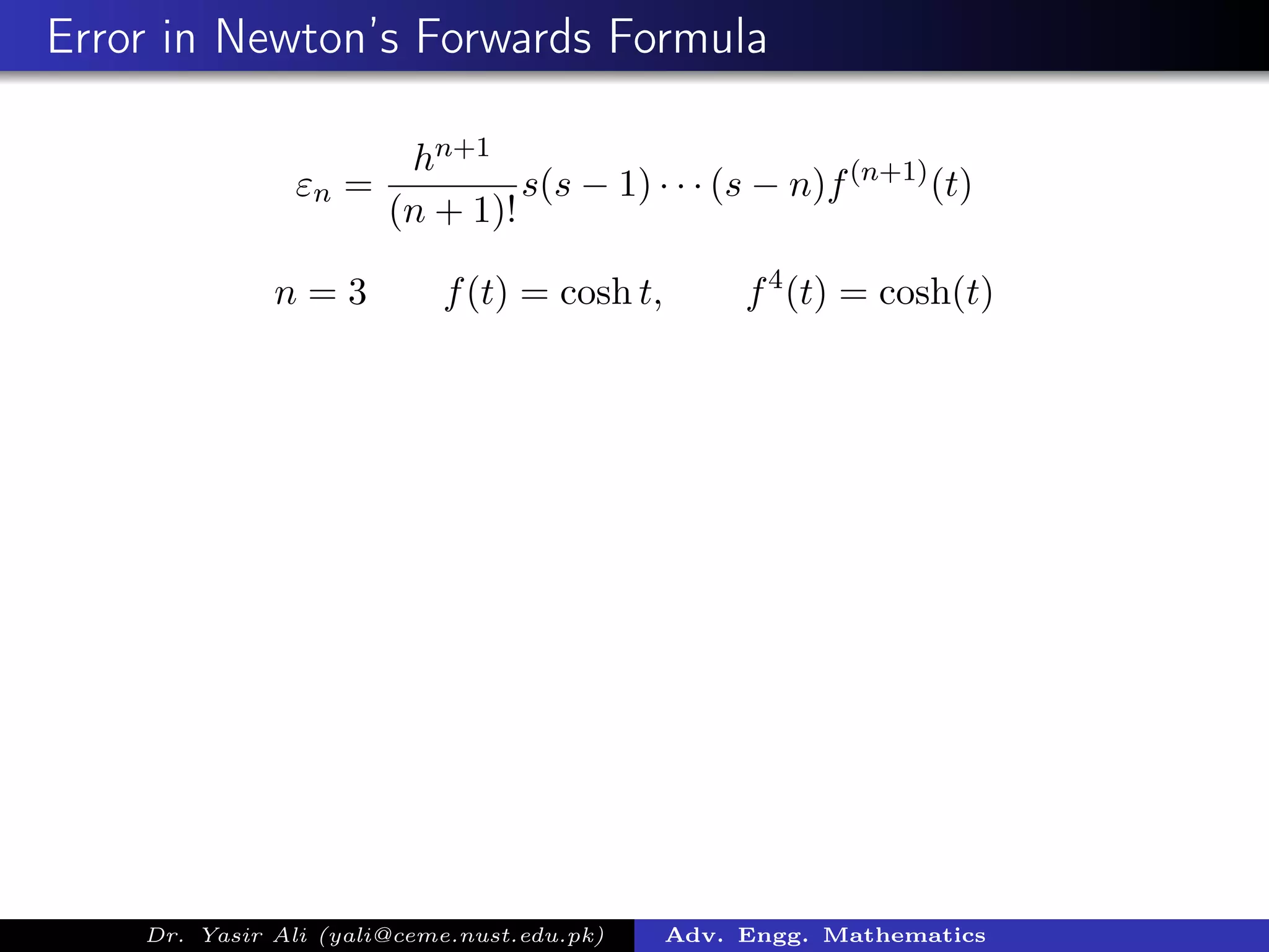
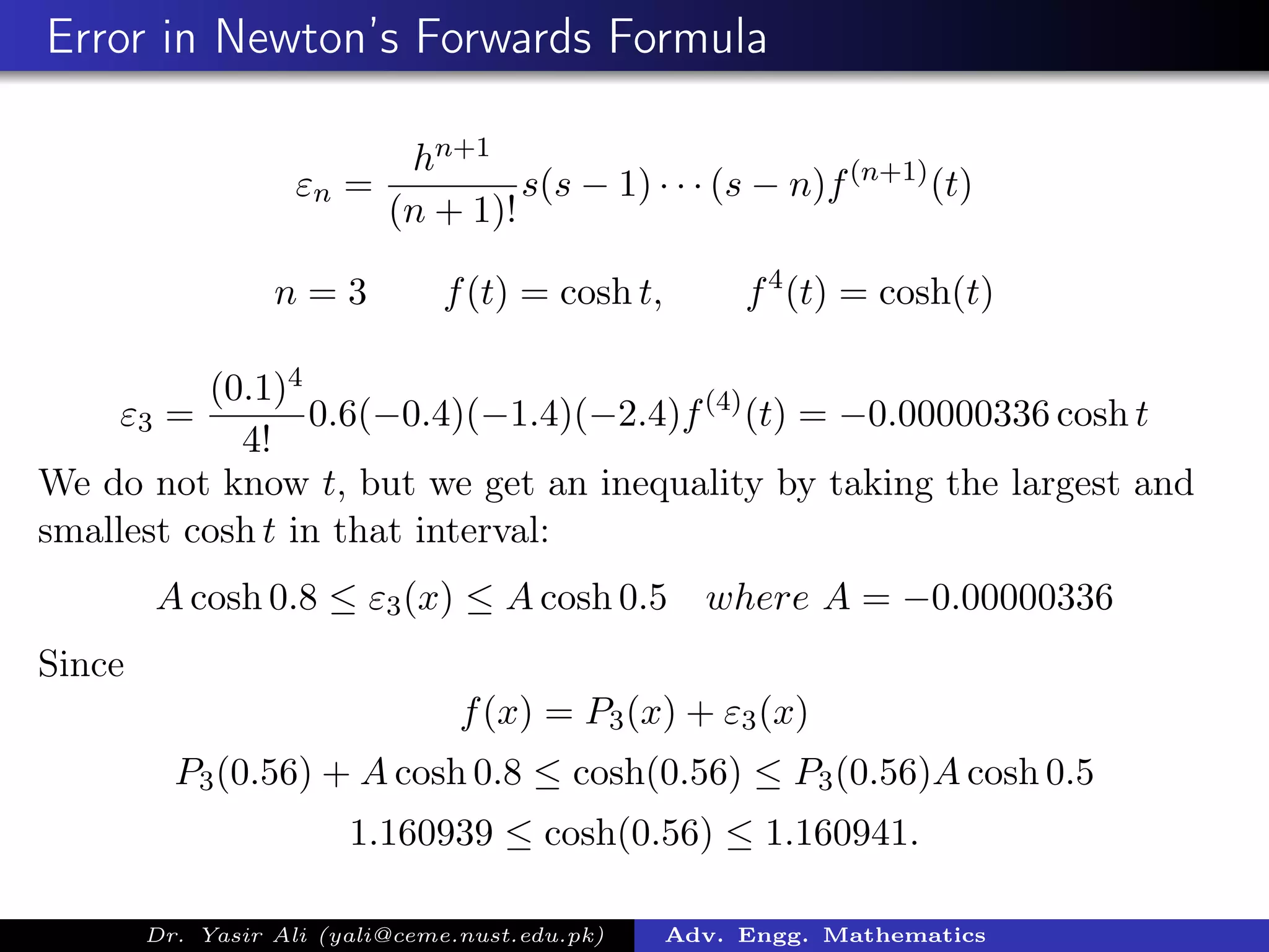
Analyzes error in the Newton’s forward formula, providing bounds for errors based on given derivatives and inputs.


![ANPARA THERMAL POWER STATION[1] sangam.pdf](https://cdn.slidesharecdn.com/ss_thumbnails/anparathermalpowerstation1sangam-251121115219-9261cde4-thumbnail.jpg?width=640&height=640&fit=bounds)


